7.3 Model & Pipeline Parallelism

In the previous section, we explored how ZeRO solves the Memory Wall by dynamically partitioning model states across a cluster. However, ZeRO has a fundamental limitation: it operates at the layer level. During a forward or backward pass, ZeRO must reconstruct the entire weight matrix of a specific layer on a single GPU.

As Foundation Models scale beyond 100 billion parameters, the mathematical operations themselves become too colossal. For a sufficiently large model or an extremely long context window, the activations and weights of a single layer will exceed the 80GB VRAM limit of an H100 GPU. When a single matrix multiplication cannot fit into memory, Data Parallelism (even with ZeRO) fails. We must physically shard the model itself.

This brings us to the two pillars of model sharding: Pipeline Parallelism (Inter-layer) and Tensor Parallelism (Intra-layer).

1. Pipeline Parallelism (PP)

Pipeline Parallelism treats the neural network like a factory assembly line. Instead of placing the entire model on one GPU, we slice the model by depth. For a 40-layer Transformer on 4 GPUs, GPU 0 handles layers 1-10, GPU 1 handles layers 11-20, and so on.

The Bubble Problem and Micro-batching

The naive approach to PP is disastrous for hardware utilization. If GPU 0 processes a batch and sends it to GPU 1, GPU 0 sits idle until the backward pass returns. This idle time is known as the Pipeline Bubble.

To mitigate this, Google introduced GPipe [1]. GPipe divides a large mini-batch into smaller micro-batches. GPU 0 processes Micro-batch 1 ($F_1$) and immediately passes it to GPU 1. While GPU 1 works on $F_1$, GPU 0 can start processing $F_2$. This keeps the pipeline “full” and drastically shrinks the relative size of the bubble.

1F1B (One-Forward-One-Backward)

While GPipe solves the utilization problem, it creates a severe memory problem. GPipe executes all forward micro-batches before executing any backward micro-batches. This means GPU 0 must store the activations for every single micro-batch in memory until the backward pass eventually arrives.

Modern frameworks (like Megatron-LM) replace GPipe with the 1F1B (One-Forward-One-Backward) schedule. In 1F1B, as soon as the last GPU finishes a forward pass for a micro-batch, it immediately executes the backward pass. This backward pass propagates up the pipeline, interleaving with forward passes.

By running backward passes early, 1F1B frees the activation memory immediately. While the pipeline bubble size remains mathematically identical to GPipe, the peak memory footprint is drastically reduced, bounded only by the number of pipeline stages rather than the number of micro-batches.

Interactive Visualization: GPipe vs 1F1B

Use the visualizer below to compare the GPipe and 1F1B schedules. Pay close attention to the Peak Memory chart at the bottom, which tracks how many micro-batch activations GPU 0 must hold in memory at any given time.

2. Tensor Parallelism (TP)

While Pipeline Parallelism splits the model between layers, Tensor Parallelism (TP) splits the mathematical operations inside a single layer.

Spearheaded by NVIDIA’s Megatron-LM [2], TP is the engine that makes training massive models possible. It physically slices the weight matrices of the Multi-Head Attention (MHA) and Multi-Layer Perceptron (MLP) blocks across multiple GPUs.

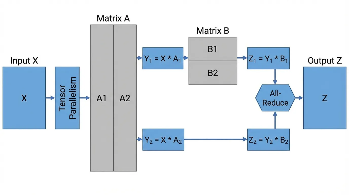Source: AI-generated illustration. Inspired by Shoeybi et al., 2019.

The Megatron-LM MLP Split

A standard Transformer MLP consists of two linear transformations: $Y = \text{GeLU}(XA)$ and $Z = YB$. Megatron-LM uses a brilliant combination of Column Parallelism and Row Parallelism to distribute this computation while minimizing communication.

1. Column Parallelism on $A$: The first weight matrix $A$ is split vertically into $A_1$ and $A_2$. GPU 0 computes $Y_1 = XA_1$ and GPU 1 computes $Y_2 = XA_2$. Because the non-linear GeLU activation is element-wise, it can be applied independently on each GPU. Zero communication is required so far.
2. Row Parallelism on $B$: The second weight matrix $B$ is split horizontally into $B_1$ and $B_2$. GPU 0 computes $Z_1 = Y_1 B_1$ and GPU 1 computes $Z_2 = Y_2 B_2$.
3. Synchronization: The final output requires summing the partial results: $Z = Z_1 + Z_2$. This is achieved via a single All-Reduce operation.

TP Process Groups and Autograd

The equations above are correct, but a raw in-place dist.all_reduce is not a realistic training implementation. A correct tensor-parallel layer must satisfy all of these contracts:

• create a TP process group containing only the ranks for one tensor-parallel replica; the global group would mix data- and pipeline-parallel replicas;
• use framework tensor-parallel APIs or autograd-aware collective mappings so the backward pass applies the matching split, gather, reduce, or identity transformation;
• assert that hidden, head, and feed-forward dimensions are divisible by the TP degree and shard the intended weight axis;
• add the row-parallel output bias exactly once after the partial sums are reduced; a replicated bias inside every local linear layer would be multiplied by the TP size;
• initialize or load slices from one canonical full weight and compare forward outputs plus input/parameter gradients against a single-device reference.

PyTorch’s tensor-parallel interfaces and established frameworks encode these mappings; they should be preferred to an educational hand-written collective [5]. Profile the actual TP subgroup and topology, because collective latency and overlap—not the word “all-reduce”—determine whether intra- or inter-node TP is viable.

The Communication Bottleneck

Tensor parallelism introduces collectives inside Transformer blocks, so latency, message size, topology, and overlap matter. High-bandwidth intra-node fabrics are often the first placement choice, but cross-node TP can be viable on suitable fabrics and workload shapes. Measure step time, collective bytes, overlap, and stragglers for candidate TP degrees instead of treating the node boundary as an absolute rule.

3. Sequence and Context Parallelism

The term sequence parallelism is overloaded. In Megatron-style tensor parallelism, sequence parallelism commonly shards operations such as normalization and dropout along the sequence dimension, reducing replicated activation memory while pairing with TP collectives. It does not by itself make every token attend globally without communication.

Long-context systems also use context parallelism or sequence-dimension attention algorithms such as Ring Attention and Ulysses. They partition tokens for attention and exchange key/value or intermediate blocks with different collective and memory patterns. Record which definition the framework uses, which tensors are sharded, whether causal and padding masks remain correct, and the communication volume per layer. Benchmark the exact sequence length and topology rather than treating these methods as interchangeable.

4. 3D Parallelism & Automated Sharding

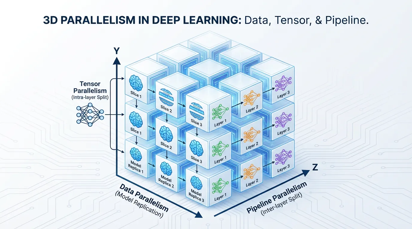
To train a state-of-the-art model like Llama 3 or GPT-4, engineers do not choose between these techniques; they combine them into 3D Parallelism.

Source: AI-generated illustration.

1. Tensor Parallelism (Intra-node): Shards the math across the 8 GPUs inside a single server using high-speed NVLink.
2. Pipeline Parallelism (Inter-node): Shards the layers across multiple servers using InfiniBand.
3. Data Parallelism (Cluster-wide): Replicates this entire TP+PP setup across thousands of servers to process massive datasets concurrently.

The Rise of Auto-Parallelism

Manually mapping a neural network to a 3D hardware topology is an agonizing engineering task. The current frontier of systems research is Automated Parallelism. Compilers like Alpa [4] treat parallelism as an optimization problem. By analyzing a computational graph and topology cost model, systems such as Alpa search for a candidate DP/TP/PP plan [4]. The result is only as accurate as the cost model and supported operators, so engineers must profile and validate it on the deployed cluster.

Quizzes

References

1. Huang, Y., et al. (2019). GPipe: Easy Scaling with Micro-Batch Pipeline Parallelism. NeurIPS. arXiv:1811.06965.
2. Shoeybi, M., et al. (2019). Megatron-LM: Training Multi-Billion Parameter Language Models Using Model Parallelism. arXiv:1909.08053.
3. Li, S., et al. (2021). Sequence Parallelism: Making 4D Parallelism Possible. arXiv:2105.13120.
4. Zheng, L., et al. (2022). Alpa: Automating Inter- and Intra-Operator Parallelism for Distributed Deep Learning. OSDI. arXiv:2201.12023.
5. PyTorch. Tensor Parallelism APIs. PyTorch documentation.