8.1 The Power Law: The Thermodynamics of Deep Learning

Before 2020, deep learning architecture design was largely driven by intuition, heuristics, and trial-and-error. Engineers would build a model, train it, and hope the loss curve converged to a satisfactory number. The paradigm shifted as researchers found repeatable empirical trends that can often be approximated by scaling laws within a defined model, data, and optimization regime.

If backpropagation is the mechanics of deep learning, scaling laws are its thermodynamics. They describe the macroscopic behavior of the system—how the final loss of a model behaves as you scale up the fundamental resources: Compute, Data, and Parameters.

This regularity lets teams use smaller pilot runs to forecast a larger run, but the forecast is conditional on the data, architecture, optimization, and extrapolation range and must carry uncertainty.

The Empirical Discovery

While early observations of predictable scaling were documented by Hestness et al. in 2017 [1], the definitive formalization for modern Large Language Models (LLMs) was published by OpenAI’s Kaplan et al. in 2020 [2].

By training dozens of Transformer models ranging from thousands to billions of parameters, they discovered that the cross-entropy test loss ($L$) decreases as a simple power law with respect to three variables, provided the other two are not acting as bottlenecks:

1. $N$ (Parameters): The number of non-embedding parameters.
2. $D$ (Data): The number of tokens trained on.
3. $C$ (Compute): The total floating-point operations (FLOPs) used during training.

The Mathematical Formulation

The power law relationship can be expressed through three independent equations:

$L(N) = \left(\frac{N_c}{N}\right)^{\alpha_N} + L_{\text{irreducible}}$

$L(D) = \left(\frac{D_c}{D}\right)^{\alpha_D} + L_{\text{irreducible}}$

$L(C) = \left(\frac{C_c}{C}\right)^{\alpha_C} + L_{\text{irreducible}}$

Where:

• $\alpha_N, \alpha_D, \alpha_C$ are the scaling exponents that dictate how fast the loss drops. Kaplan found these to be approximately $\alpha_N \approx 0.076$, $\alpha_D \approx 0.095$, and $\alpha_C \approx 0.050$.
• $N_c, D_c, C_c$ are constants representing characteristic scales.
• $L_{\text{irreducible}}$ is the inherent entropy of the dataset.

The Irreducible Loss Floor

The term $L_{\text{irreducible}}$ represents a theoretical minimum. Natural language contains inherent ambiguity, noise, and unobserved context. Even a theoretical model with infinite parameters and infinite compute cannot perfectly predict the next token every single time. As models grow exponentially larger, the returns diminish as the loss curve flattens out, asymptotically approaching this entropy floor.

Log-Log Linearity

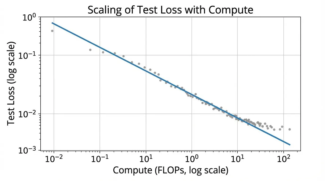
The power law is most clearly visualized on a log-log plot. If we ignore the irreducible loss for a moment (assuming we are far from the floor), taking the logarithm of the compute scaling equation yields:

$\log L(C) \approx -\alpha_C \log C + \log(C_c^{\alpha_C})$

This is the equation of a straight line ($y = mx + b$). This linearity is what makes scaling laws so powerful for engineering. You can plot the loss of a 10M, 100M, and 1B parameter model on a log-log graph, draw a straight line through them, and accurately predict the loss of a 100B parameter model.

Extrapolating with Constraints and Uncertainty

Scaling-law forecasts are engineering estimates, not exact predictions. Use the same tokenizer, data snapshot, architecture family, evaluation harness, and training-quality criteria across a factorial pilot grid of model sizes $N$, token budgets $D$, and multiple seeds. Tune learning rate, batch, and warmup for each scale rather than turning small-model under-training into an apparent scaling law.

The following educational fit constrains amplitude and exponent to be positive and the floor to lie between zero and the smallest observed loss. Compute is measured in PetaFLOPs: 1 ExaFLOP = 1,000 PetaFLOPs, so the target is 1e3, not 1e6.

import torch
import torch.nn as nn
import torch.nn.functional as F

compute_pf = torch.tensor([10., 30., 100., 300., 1_000.])
validation_loss = torch.tensor([4.65, 4.02, 3.52, 3.18, 2.91])

class ConstrainedPowerLaw(nn.Module):
    def __init__(self, min_observed_loss):
        super().__init__()
        self.raw_amplitude = nn.Parameter(torch.tensor(1.0))
        self.raw_exponent = nn.Parameter(torch.tensor(-2.0))
        self.raw_floor_fraction = nn.Parameter(torch.tensor(0.0))
        self.register_buffer("min_loss", min_observed_loss)

    def forward(self, compute):
        amplitude = F.softplus(self.raw_amplitude)
        exponent = F.softplus(self.raw_exponent)
        floor = self.min_loss * torch.sigmoid(self.raw_floor_fraction)
        return amplitude * compute.pow(-exponent) + floor

model = ConstrainedPowerLaw(validation_loss.min())
optimizer = torch.optim.Adam(model.parameters(), lr=1e-2)
for _ in range(5_000):
    prediction = model(compute_pf)
    loss = F.mse_loss(torch.log(prediction), torch.log(validation_loss))
    optimizer.zero_grad()
    loss.backward()
    optimizer.step()

one_exaflop_pf = torch.tensor([1_000.])
print(model(one_exaflop_pf).item())

Five aggregate points are still insufficient for a funding decision. Resample whole pilot runs with a bootstrap to obtain parameter and forecast intervals; do not resample individual validation tokens as if training runs were independent. Perform a leave-largest-out test: fit without the largest run and forecast it. Report that error and reject extrapolations far beyond the validated compute ratio.

Reserve the largest planned pilot scale as a genuine forecast holdout. Compare predicted and actual validation loss, downstream checkpoint probes, achieved FLOP/s, restart overhead, and total cost. Convert peak FLOPs into GPU-hours using measured utilization and include data, checkpoint, evaluation, and failure overhead. A go/no-go band should include uncertainty and business value, not only a point estimate.

The “Mirage” of Emergent Abilities

A critical nuance in scaling laws is the distinction between cross-entropy loss and downstream task accuracy.

Cross-entropy often follows a smooth trend within a fitted regime, while capabilities on specific benchmarks can appear to show sudden, discontinuous jumps. Neither behavior is guaranteed outside the measured model, data, and optimization range.

However, researchers like Schaeffer et al. (2023) [3] argue that this emergence is largely a mirage caused by the choice of metric. Cross-entropy is continuous; it measures the probability distribution over tokens. If a model improves its probability assigned to the correct answer from 1% to 10%, the loss drops smoothly. But on a multiple-choice benchmark, the model will still score 0% until that probability surpasses the competing incorrect options, at which point the accuracy suddenly spikes to 100%.

Metric choice can create or amplify apparent thresholds, as Schaeffer et al. demonstrate for studied settings [3]. That result does not settle every emergence claim; engineers should inspect continuous metrics, contamination, prompting, and confidence intervals rather than treating either smoothness or discontinuity as universal.

Quizzes

References

1. Hestness, J., et al. (2017). Deep Learning Scaling is Predictable, Empirically. arXiv:1712.00409.
2. Kaplan, J., et al. (2020). Scaling Laws for Neural Language Models. arXiv:2001.08361.
3. Schaeffer, R., et al. (2023). Are Emergent Abilities of Large Language Models a Mirage?. arXiv:2304.15004.