1.2 The Power of Representation

The true breakthrough of Deep Learning, which enables modern foundation models, is not just that networks are bigger, but that they solve the problem of Representation.

Motivation: Why Representation is Everything

In AI, how you represent data determines what the model can learn.

Breaking the Curse of Dimensionality: Raw data (like a 4K image) has too many dimensions for traditional algorithms. Good representations reduce this to a small, manageable set of features.
Generalization: A good representation captures the essence of the data (e.g., the concept of a “dog” rather than specific pixel values), allowing the model to perform well on new, unseen data.
Foundation Models: Modern models like GPT-4 or Gemini are essentially massive representation learners. They learn a universal representation of language and the world, which can then be used for thousands of different tasks.

The Metaphor: Describing a Face vs. Recognizing a Face

Imagine you need to identify a person in a crowd.

Feature Engineering (The Old Way) is like trying to describe the person over the phone. You might say: “They have a nose that is 2 inches long, eyes that are 1.5 inches apart, and a round chin.” You are manually extracting specific features. If you measure the wrong thing, or if the person turns their head, the description fails.
Representation Learning (Deep Learning) is like looking at the person’s photo. Your brain doesn’t measure nose length. It processes the whole image and extracts a high-level, abstract representation of “that person’s face.” It works even if the lighting changes or they wear glasses.

Deep Learning succeeded because it stopped asking humans to describe the features and let the system discover the best representation on its own.

The Paradigm Shift: Statistics vs. Machine Learning

To understand why AI moved from hand-crafted rules (Symbolism) to learning representations (Deep Learning), we must understand the shift in philosophy from traditional statistics to machine learning. This is what Leo Breiman famously called the “Two Cultures” of statistical modeling [3].

The Statistical Culture (Inference): Traditional statistics focuses on understanding the relationship between variables. It assumes a stochastic data model (like linear regression) and focuses on parameters, p-values, and confidence intervals. It works well with small data and prioritizes interpretability and causality.
The Machine Learning Culture (Prediction): Machine learning treats the data mechanism as unknown and focuses on finding an algorithm that can accurately predict output $y$ from input $x$ . It prioritizes prediction accuracy and generalization on unseen data, often using complex, non-linear models (like neural networks) that operate as “black boxes.”

Deep Learning and Foundation Models are the ultimate evolution of the Machine Learning culture. They prioritize empirical performance on massive scale over traditional statistical interpretability. Understanding this shift helps explain why LLMs are incredibly capable yet hard to explain mathematically in terms of exact rules.

A Brief History: From Hand-Crafted Features to Deep Learning

The history of machine learning can be viewed as an evolution in how we represent data.

The Hand-Crafted Era (Pre-2012): For decades, domain experts designed features manually. In computer vision, we used SIFT or HOG. In NLP, we used TF-IDF or carefully constructed dictionaries. This was slow, brittle, and required extreme domain expertise.
The Deep Learning Breakthrough (2012): AlexNet won the ImageNet competition by a huge margin. It didn’t use hand-crafted features; it learned them directly from pixels using a deep convolutional neural network. This proved that automated representation learning outperforms human design.
The Self-Supervised Era (2018-Present): Models like BERT and GPT showed that by predicting missing words in massive amounts of text, models can learn incredibly rich representations of language without human labels.

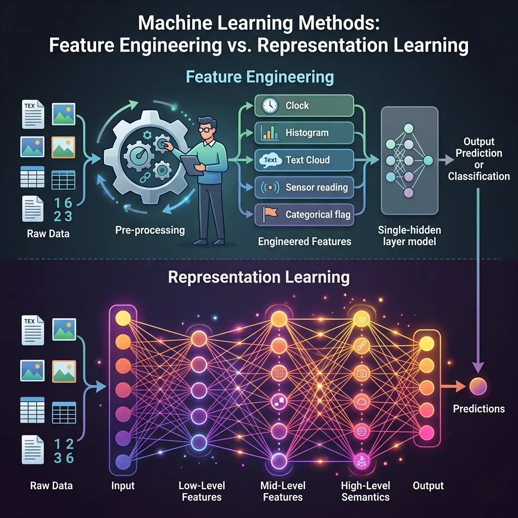
Feature Engineering vs Representation Learning

Source: Generated by AI

Feature Engineering vs. Representation Learning

Feature	Feature Engineering (Traditional ML)	Representation Learning (Deep Learning)
Who designs features?	Human experts	The algorithm (Neural Network)
Domain Specificity	High (Needs experts for every field)	Low (Same architecture works for many fields)
Scalability	Low (Labor intensive)	High (Scales with data and compute)
Interpretability	High (We know exactly what features are)	Low (Black box representations)
Performance	Limited by human intuition	SOTA on complex tasks

The Manifold Hypothesis

A key theoretical concept in representation learning is the Manifold Hypothesis.

It posits that real-world high-dimensional data (like all possible $256 \times 256$ images) actually lies on a much lower-dimensional, non-linear subspace (a manifold) embedded within the high-dimensional space.

Think of a crumpled piece of paper. It exists in 3D space, but the paper itself is a 2D surface. The goal of representation learning is to “uncrumple” the paper to understand the data better, finding the true underlying factors of variation.

Learning a Latent Space

Let’s see this in code. One of the simplest ways to see representation learning is through an Autoencoder. An autoencoder compresses input data into a lower-dimensional “latent space” (representation) and then tries to reconstruct the original input.

Here is a PyTorch implementation of a simple Autoencoder learning a representation of data.

import torch
import torch.nn as nn
import torch.optim as optim

# Generate dummy high-dimensional data (e.g., 10-dimensional)
# But let's make it actually depend on just 2 underlying factors
N = 1000
latent_dim = 2
data_dim = 10

torch.manual_seed(42)
true_latent = torch.randn(N, latent_dim)
# Project to high dimension with some non-linearity
projection = nn.Linear(latent_dim, data_dim)
with torch.no_grad():
    X = torch.sin(projection(true_latent)) + torch.randn(N, data_dim) * 0.1

# Autoencoder Model
class Autoencoder(nn.Module):
    def __init__(self):
        super(Autoencoder, self).__init__()
        # Encoder: compresses to 2D
        self.encoder = nn.Sequential(
            nn.Linear(data_dim, 5),
            nn.ReLU(),
            nn.Linear(5, latent_dim)
        )
        # Decoder: reconstructs back to 10D
        self.decoder = nn.Sequential(
            nn.Linear(latent_dim, 5),
            nn.ReLU(),
            nn.Linear(5, data_dim)
        )

    def forward(self, x):
        latent = self.encoder(x)
        reconstructed = self.decoder(latent)
        return reconstructed, latent

model = Autoencoder()
criterion = nn.MSELoss()
optimizer = optim.Adam(model.parameters(), lr=0.01)

# Training
for epoch in range(1000):
    reconstructed, latent = model(X)
    loss = criterion(reconstructed, X)
    
    optimizer.zero_grad()
    loss.backward()
    optimizer.step()
    
    if (epoch + 1) % 200 == 0:
        print(f'Epoch [{epoch+1}/1000], Loss: {loss.item():.4f}')

print("Model learned to compress 10D data into a 2D representation!")

Example: Feature Engineering vs. Representation Learning in NLP

Compare how Traditional ML (Lexicon-based Feature Engineering) and Deep Learning (Representation Learning) handle context and sentiment in natural language.

Feature Engineering vs Representation Learning in NLP

See how different paradigms handle context and sentiment.

Select a Sentence:

Feature Engineering (Lexicon Based)

Word Counts:

Positive Words: good

Negative Words: None

Rule: Sum scores (+1 for pos, -1 for neg)

Score: 1

Classification: Positive

Representation Learning (Latent Space)

Semantic Mapping:

Positive Region

Negative Region

Classification: Positive

Insight: Simple positive sentence. Both methods easily identify the sentiment.

Quizzes

Quiz 1: What is the main difference between Feature Engineering and Representation Learning?

In Feature Engineering, human experts manually design and extract relevant features from raw data before feeding them into a model. In Representation Learning, the model automatically learns to extract these features directly from the raw data during training, typically through multiple layers of abstraction in a deep network.

Quiz 2: How does the Manifold Hypothesis explain why high-dimensional data can be processed by smaller networks?

The Manifold Hypothesis suggests that although data may exist in a high-dimensional space (e.g., millions of pixels), the actual meaningful variation in the data lies on a much lower-dimensional manifold. By learning to project the data onto this manifold, representation learning reduces the effective dimensionality, allowing simpler models or subsequent layers to process it effectively.

Quiz 3: Give an example of hierarchical representation in Natural Language Processing.

In NLP, lower levels might represent raw characters or sub-word tokens. The next level combines them into words or morphemes. Higher levels represent phrases, then sentences, and finally full document concepts or intents. Modern LLMs learn these hierarchies implicitly through their attention layers.

Quiz 4: Why is Self-Supervised Learning considered a major milestone in Representation Learning?

Self-supervised learning allows models to learn representations from unlabeled data by creating pretext tasks (like predicting masked words or next frames). This eliminates the need for massive human-labeled datasets, which were a major bottleneck, enabling models to train on internet-scale data and learn universal representations.

Quiz 5: What are the risks of relying entirely on automated Representation Learning in high-stakes domains (e.g., healthcare)?

The primary risks are lack of interpretability and bias amplification. Since the model learns its own representations, it is difficult for humans to understand why it made a specific decision (the black box problem). If the training data contains biases, the model will learn to represent those biases, potentially leading to unfair or dangerous outcomes.

Quiz 6: Derive the analytical gradient of the Mean Squared Error (MSE) loss with respect to the bottleneck latent representation

\mathbf{z}

in an Autoencoder.

Let $\mathbf{x}$ be the input, $\mathbf{z} = f_\theta(\mathbf{x})$ be the bottleneck representation, and $\mathbf{\hat{x}} = g_\phi(\mathbf{z})$ be the reconstruction. The MSE loss is $L = \frac{1}{D} \sum_{i=1}^D (x_i - \hat{x}_i)^2 = \frac{1}{D} \|\mathbf{x} - \mathbf{\hat{x}}\|^2_2$ . By the chain rule, the gradient with respect to the latent vector $\mathbf{z}$ is: $\frac{\partial L}{\partial \mathbf{z}} = \frac{\partial L}{\partial \mathbf{\hat{x}}} \frac{\partial \mathbf{\hat{x}}}{\partial \mathbf{z}}$ . We know $\frac{\partial L}{\partial \mathbf{\hat{x}}} = -\frac{2}{D} (\mathbf{x} - \mathbf{\hat{x}})$ . Therefore, $\frac{\partial L}{\partial \mathbf{z}} = -\frac{2}{D} (\mathbf{x} - \mathbf{\hat{x}})^T \mathbf{J}_g(\mathbf{z})$ , where $\mathbf{J}_g(\mathbf{z}) = \frac{\partial g_\phi(\mathbf{z})}{\partial \mathbf{z}}$ is the Jacobian matrix of the decoder function $g_\phi$ evaluated at $\mathbf{z}$ .

References

Bengio, Y., Courville, A., & Vincent, P. (2013). Representation learning: A review and new perspectives. IEEE transactions on pattern analysis and machine intelligence, 35(8), 1798-1828. arXiv:1206.5538.
LeCun, Y., Bengio, Y., & Hinton, G. (2015). Deep learning. Nature, 521(7553), 436-444.
Breiman, L. (2001). Statistical modeling: The two cultures. Statistical science, 16(3), 199-231.
Recommended Video: StatQuest: Word Embedding and Word2Vec A great visual explanation of Word Embeddings and Word2Vec, a prime example of representation learning.