19.3 Probing Classifiers

The Logit Lens from the previous section is a powerful tool, but it suffers from a fundamental limitation: it only reveals what the model is about to output. By mapping the residual stream directly to the vocabulary space via the unembedding matrix, we are strictly looking at the model’s immediate predictive intent.

But what if the model possesses knowledge that it isn’t explicitly verbalizing?

• Does the model know that the subject of a sentence is plural, even if the next predicted word isn’t a verb?
• Does the model internally know a statement is factually false, even while it is being prompted to generate a lie?
• Is a concept like “sarcasm” or “sentiment” explicitly tracked in the hidden states?

To answer these questions, we cannot rely on the unembedding matrix. Instead, we must interrogate the model’s internal representations directly. We do this by training an auxiliary classifier—a Probe—on the frozen hidden states of the model.

1. The Interrogation Room: What is a Probe?

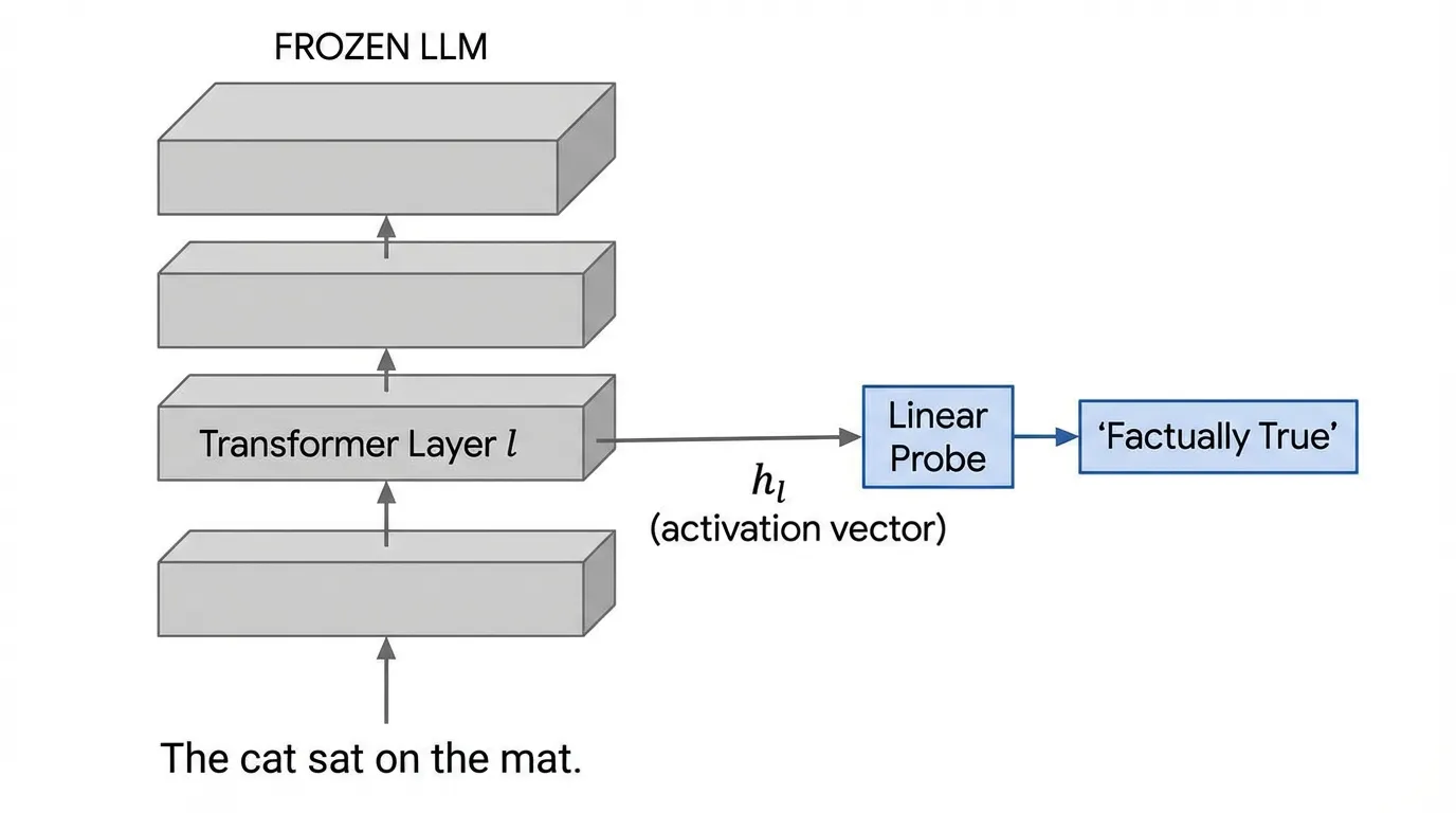
The core idea of probing is to treat a pre-trained, frozen Large Language Model as a feature extractor. We run a dataset of inputs $X$ through the model and extract the continuous activation vectors $h_l \in \mathbb{R}^d$ at a specific layer $l$.

We then train a secondary, lightweight supervised model (the probe) $f_\theta: \mathbb{R}^d \rightarrow \mathcal{Y}$ to predict a specific property $Y$ (e.g., Part-of-Speech, syntactic depth, or factual truth) from those activations.

Source: Generated by Gemini

If the probe achieves high accuracy, we conclude that the information required to predict property $Y$ is encoded within the representations at layer $l$.

2. The Linear Representation Hypothesis

When designing a probe, a critical question arises: How complex should the probe be?

If we use a deep, highly parameterized Multi-Layer Perceptron (MLP) as our probe, it could easily achieve 100% accuracy. However, a powerful MLP might just be learning the task itself from the raw data, completely bypassing the LLM’s internal structure. In this scenario, the probe isn’t reading the LLM’s mind; it’s doing the thinking for it.

To prevent this, researchers overwhelmingly rely on the Linear Representation Hypothesis (LRH) [1]. The LRH posits that modern neural networks encode high-level semantic concepts as linear directions (or hyperplanes) within their high-dimensional activation space.

Therefore, standard practice dictates using Linear Probes (e.g., Logistic Regression or a single linear layer). The mathematical formulation is intentionally constrained:

$\hat{y} = \text{argmax}(\text{softmax}(W \cdot h_l + b))$

If a simple linear hyperplane can successfully separate complex concepts (e.g., true statements from false statements), it serves as strong evidence that the LLM has already done the heavy computational lifting to extract and organize that concept by layer $l$.

3. Engineering a Linear Probe (PyTorch)

Training a probe involves two distinct phases: extracting the activations from the frozen LLM, and training the linear classifier. Below is a realistic PyTorch implementation demonstrating how to train a linear probe on pre-extracted activations.

import torch
import torch.nn as nn
from torch.utils.data import DataLoader, TensorDataset

class LinearProbe(nn.Module):
    """
    A strictly linear probe to test the Linear Representation Hypothesis.
    No hidden layers, no non-linear activation functions.
    """
    def __init__(self, input_dim: int, num_classes: int):
        super().__init__()
        self.proj = nn.Linear(input_dim, num_classes)
        
    def forward(self, x: torch.Tensor) -> torch.Tensor:
        # Output raw logits
        return self.proj(x)

def train_probe(activations: torch.Tensor, labels: torch.Tensor, epochs: int = 10) -> nn.Module:
    """
    Trains a linear probe on frozen LLM activations.
    
    Args:
        activations: Tensor of shape (N, hidden_dim) extracted from layer l.
        labels: Tensor of shape (N,) containing target concept classes.
    """
    # 1. Prepare data loaders
    dataset = TensorDataset(activations, labels)
    loader = DataLoader(dataset, batch_size=64, shuffle=True)
    
    input_dim = activations.shape[-1]
    num_classes = labels.max().item() + 1
    
    # 2. Initialize the probe and optimizer
    # Weight decay is crucial here to prevent the linear probe from overfitting
    # to spurious noise directions in the high-dimensional space.
    probe = LinearProbe(input_dim, num_classes).to(activations.device)
    optimizer = torch.optim.AdamW(probe.parameters(), lr=1e-3, weight_decay=0.01)
    criterion = nn.CrossEntropyLoss()
    
    # 3. Training Loop
    probe.train()
    for epoch in range(epochs):
        total_loss = 0.0
        correct = 0
        total = 0
        
        for batch_x, batch_y in loader:
            optimizer.zero_grad()
            
            logits = probe(batch_x)
            loss = criterion(logits, batch_y)
            
            loss.backward()
            optimizer.step()
            
            total_loss += loss.item()
            predictions = torch.argmax(logits, dim=-1)
            correct += (predictions == batch_y).sum().item()
            total += batch_y.size(0)
            
        print(f"Epoch {epoch+1} | Loss: {total_loss/len(loader):.4f} | Acc: {correct/total:.4f}")
            
    return probe

4. The Selectivity Problem: Is the Probe Cheating?

Even with a strictly linear probe, there is a risk that the probe is memorizing the dataset rather than uncovering latent, generalized knowledge. Hewitt and Liang (2019) formalized this as the Selectivity Problem [2].

To prove a probe is actually reading the LLM’s structural knowledge, they introduced the concept of Control Tasks.

• Real Task: Train a probe to predict the actual Part-of-Speech (POS) of words from their activations.
• Control Task: Assign a random, deterministic label to each word type (e.g., every instance of the word “apple” is assigned class 3, “run” is class 1) and train a probe to predict it.

If the probe achieves 90% accuracy on the Real Task and 85% on the Control Task, the probe is simply memorizing word identities (mapping specific token embeddings to arbitrary labels). A high-quality probe must exhibit high Selectivity, defined as:

$\text{Selectivity} = \text{Accuracy}_{\text{Task}} - \text{Accuracy}_{\text{Control}}$

A high selectivity score proves that the LLM’s geometry naturally clusters the semantic concept, making the real task inherently easier to linearly separate than the random control task.

5. From Correlation to Causation: Amnesic Probing

Suppose our linear probe successfully finds a direction vector $W$ that perfectly classifies plural vs. singular subjects with high selectivity. Does this mean the LLM actually uses this information to predict the next word?

Not necessarily. The information might just be a correlated byproduct of the network’s processing. To prove causation, we must intervene in the model’s computational graph.

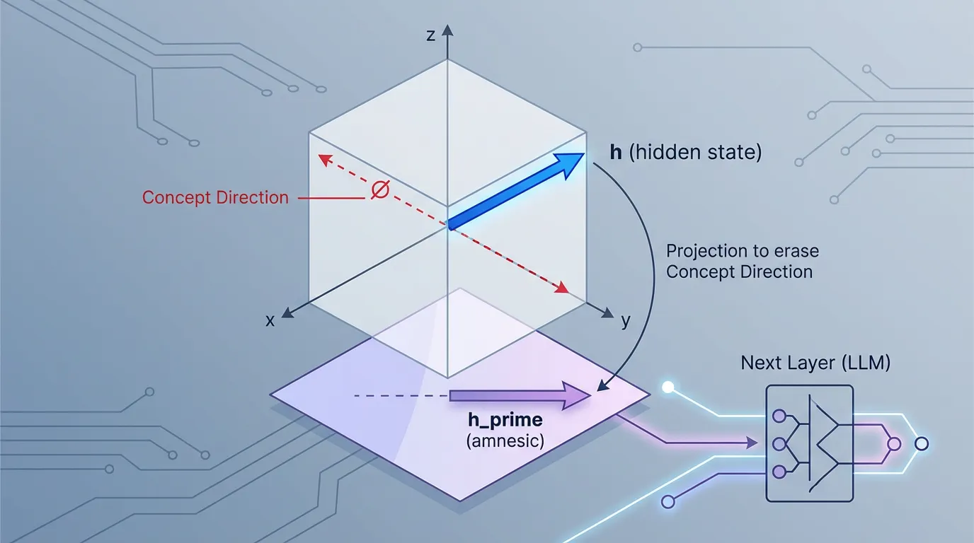
Elazar et al. (2021) introduced Amnesic Probing [3]. The methodology involves surgically removing the concept from the model’s hidden state and observing if its downstream behavior changes. This is achieved using Iterative Null-space Projection (INLP).

Mathematically, if $W$ is the weight matrix of our linear probe, we project the model’s hidden state $h_l$ onto the null space of $W$:

$h'_l = \left( I - W^T(WW^T)^{-1}W \right) h_l$

Source: Generated by Gemini

This new vector $h'_l$ contains exactly zero information about the probed concept (if fed into the probe, it would output random noise). If we substitute $h_l$ with $h'_l$ during the LLM’s forward pass, and the model suddenly fails to maintain subject-verb agreement in its generated text, we have proven a causal link: the model relies on that specific linear direction to perform the task.

6. Discovering Latent Truth (Unsupervised Probing)

One of the most profound applications of probing is discovering whether an LLM “knows” it is hallucinating.

Burns et al. (2022) proposed a method to find the “Truth Direction” in an LLM without any labeled data [4]. They introduced Contrast-Consistent Search (CCS). The intuition is based on logical consistency. If we feed the model a statement $x^+$ (“The earth is flat”) and its exact negation $x^-$ (“The earth is not flat”), we get two activation vectors $h^+$ and $h^-$.

Even without knowing which statement is factually true, we know that a valid “truth probe” $P_{true}(x)$ must satisfy the logical constraint:

$P_{true}(x^+) + P_{true}(x^-) = 1$

By training a linear probe to simply minimize this consistency loss across thousands of paired statements, the probe naturally converges on the latent “truth direction” inside the LLM. This remarkable finding allows researchers to detect when a model is lying, even if the model’s standard output is explicitly prompted to generate false information.

7. Interactive: The Linear Representation Hypothesis

To visualize how concepts crystallize in the activation space, interact with the simulation below. It demonstrates how the representations of two concepts (e.g., True vs. False statements) evolve across the layers of a Transformer.

Notice how the concepts are entangled in early layers (making linear separation impossible), but naturally organize into linearly separable clusters in the deeper layers, validating the Linear Representation Hypothesis.

9. Summary and Open Questions

Probing Classifiers have allowed us to move beyond simply observing the final outputs of an LLM. By treating the network as a feature extractor, we can prove that models internally track complex linguistic, syntactical, and factual concepts long before the final token is generated. Furthermore, causal interventions like Amnesic Probing prove that the model actively relies on these internal linear geometries.

However, probing has a blind spot. A linear probe can only find a concept if we already know what we are looking for. We must provide the dataset (e.g., POS tags, true/false statements) to train the probe.

But what about the thousands of other features the LLM has learned that we haven’t thought to probe for? How can we discover the complete dictionary of concepts an LLM uses, without relying on human-defined labels?

To solve this unsupervised discovery problem, we must turn to the cutting edge of mechanistic interpretability: 19.4 Sparse Autoencoders (SAE).

Quizzes

References

1. Park, K., et al. (2023). The Linear Representation Hypothesis and the Geometry of Large Language Models. arXiv:2311.03658.
2. Hewitt, J., & Liang, P. (2019). Designing and Interpreting Probes with Control Tasks. EMNLP 2019. Link.
3. Elazar, Y., et al. (2021). Amnesic Probing: Behavioral Explanation with Amnesic Counterfactuals. Transactions of the Association for Computational Linguistics (TACL). Link.
4. Burns, C., et al. (2022). Discovering Latent Knowledge in Language Models Without Supervision. arXiv:2212.03827.