11.2 Audio & Speech Integration

Text is clean, discrete, and highly compressed. It acts like sheet music, explicitly detailing what notes to play. Audio, on the other hand, is the actual orchestral performance. It is a messy, continuous stream of high-dimensional data containing not just the words spoken, but the speaker’s identity, emotional state, prosody, and the acoustic environment.

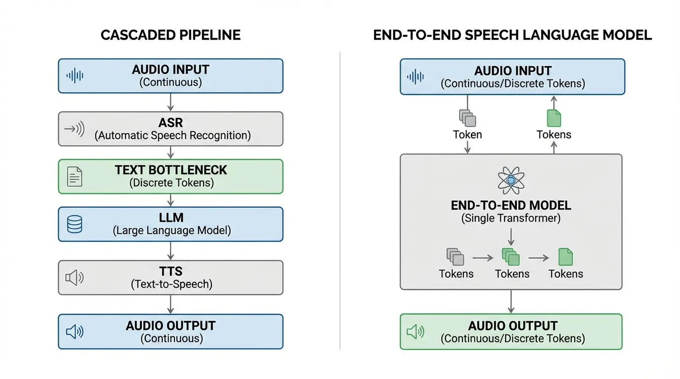
For decades, AI systems handled speech through a rigid, cascaded pipeline: Automatic Speech Recognition (ASR) to convert audio to text, a Language Model (LLM) to process the text, and Text-to-Speech (TTS) to convert the response back to audio. This cascaded approach creates an “emotion bottleneck.” The moment speech is transcribed into text, all paralinguistic information (tone, hesitation, background context) is irreversibly lost.

The modern paradigm of Foundation Models treats audio as a first-class citizen. By discretizing audio into tokens or directly modeling continuous audio spaces, we can train LLMs to “hear” and “speak” natively. This section dissects the engineering and mathematics behind integrating speech into large language models, tracing the evolution from discrete neural codecs to state-of-the-art Continuous Audio Language Models (CALM).

Source: Generated by Gemini.

1. The Modality Gap and Neural Audio Codecs

The fundamental challenge of audio language modeling is the sampling rate. A standard 16 kHz audio file contains 16,000 continuous float values per second. A text LLM processes roughly 3 to 4 discrete tokens per second. Feeding raw waveforms directly into a Transformer yields a sequence length that instantly exhausts the attention mechanism’s memory capacity.

To bridge this gap, engineers utilize Neural Audio Codecs (e.g., SoundStream, EnCodec). These models act as tokenizers for sound. They compress the high-dimensional waveform into a low frame-rate sequence of discrete tokens using a technique called Residual Vector Quantization (RVQ).

The Mathematics of RVQ

Standard Vector Quantization (VQ) maps an input vector to the nearest vector in a single learned codebook. However, a single codebook large enough to capture the vast variance of human speech would be computationally intractable. RVQ solves this by cascading multiple small codebooks.

Given an encoded continuous audio frame $x \in \mathbb{R}^d$ and $Q$ codebooks $C_1, C_2, \dots, C_Q$, where each codebook contains $N$ vectors of dimension $d$.

1. Initialize the residual: $x_1 = x$
2. For each quantizer stage $q$ from $1$ to $Q$:
   • Find the nearest codebook vector: $i_q = \arg\min_{i \in \{1 \dots N\}} \| x_q - C_q[i] \|_2^2$
   • Retrieve the quantized vector: $\hat{x}_q = C_q[i_q]$
   • Update the residual for the next stage: $x_{q+1} = x_q - \hat{x}_q$
3. The final reconstructed vector is the sum of the quantized vectors: $\hat{x} = \sum_{q=1}^Q \hat{x}_q$

The first few codebooks capture the most prominent features (semantic content, broad phonetic structure), while deeper codebooks capture the residual fine-grained details (timbre, background noise).

Engineering the Quantizer

Below is a realistic PyTorch implementation of an RVQ module. Notice how the distances are computed efficiently using the expanded quadratic formula $(x-y)^2 = x^2 + y^2 - 2xy$.

import torch
import torch.nn as nn

class ResidualVectorQuantizer(nn.Module):
    def __init__(self, num_quantizers=8, codebook_size=1024, dim=128):
        """
        Args:
            num_quantizers: Number of cascaded codebooks (Q)
            codebook_size: Number of vectors per codebook (N)
            dim: Dimension of each vector (d)
        """
        super().__init__()
        self.num_quantizers = num_quantizers
        self.codebooks = nn.ParameterList([
            nn.Parameter(torch.randn(codebook_size, dim)) 
            for _ in range(num_quantizers)
        ])
        
    def forward(self, x):
        # x shape: [batch_size, seq_len, dim]
        residual = x
        quantized_out = torch.zeros_like(x)
        token_indices = []
        
        for i in range(self.num_quantizers):
            codebook = self.codebooks[i]
            
            # Compute squared L2 distance: x^2 + y^2 - 2xy
            # residual^2: [batch, seq, 1]
            # codebook^2: [codebook_size]
            # matmul: [batch, seq, codebook_size]
            dist = (
                residual.pow(2).sum(dim=-1, keepdim=True) 
                + codebook.pow(2).sum(dim=-1) 
                - 2 * torch.matmul(residual, codebook.t())
            )
            
            # Find index of the closest codebook vector
            indices = torch.argmin(dist, dim=-1) # [batch_size, seq_len]
            token_indices.append(indices)
            
            # Lookup quantized vectors and accumulate
            quantized = codebook[indices]
            quantized_out += quantized
            
            # Update residual for the next quantizer stage
            residual = residual - quantized
            
        # token_indices shape: [batch_size, num_quantizers, seq_len]
        return quantized_out, torch.stack(token_indices, dim=1)

# Example execution simulating a 50Hz audio frame rate
batch_size = 2
seq_len = 50 # 1 second of audio
dim = 128

dummy_audio_features = torch.randn(batch_size, seq_len, dim)
rvq = ResidualVectorQuantizer(num_quantizers=8, codebook_size=1024, dim=128)
reconstructed, indices = rvq(dummy_audio_features)

print(f"Original features: {dummy_audio_features.shape}")
print(f"Reconstructed features: {reconstructed.shape}")
print(f"Token indices shape: {indices.shape}") 
# Output: -> 8 tokens per frame

2. The Pioneers: AudioLM and VALL-E

Once audio is tokenized, it can be treated like text. However, predicting audio tokens autoregressively introduces a severe trade-off between semantic coherence and acoustic fidelity.

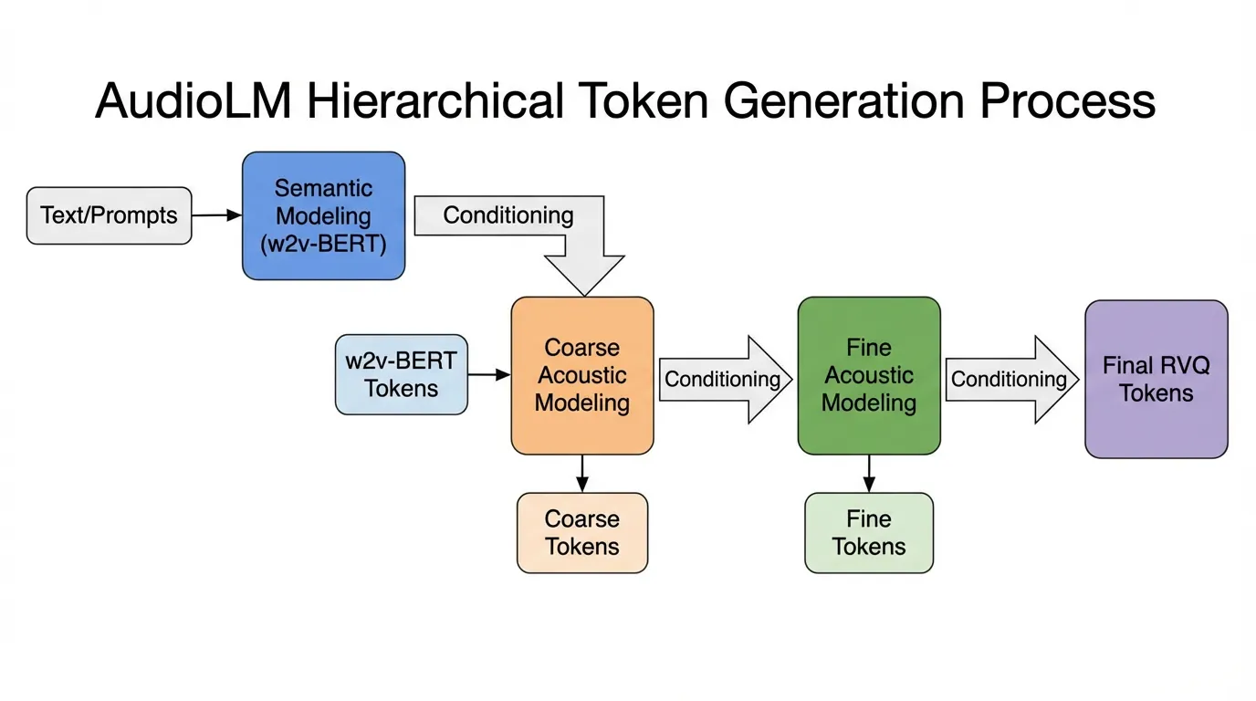
Hierarchical Tokenization (AudioLM)

Google’s AudioLM [1] solved this by decoupling “what is being said” from “how it is being said.” It utilizes two distinct types of tokens:

1. Semantic Tokens: Extracted from a self-supervised model like w2v-BERT. These tokens capture linguistic structure and phonetic content but discard speaker identity. They have a low bitrate.
2. Acoustic Tokens: Extracted from a neural codec (SoundStream). These capture the high-fidelity acoustic details.

AudioLM models the sequence hierarchically: it first autoregressively predicts the semantic tokens to ensure long-term linguistic coherence, and then uses those semantic tokens to condition the generation of the acoustic tokens, ensuring high-fidelity output.

Zero-Shot TTS as Language Modeling (VALL-E)

Microsoft’s VALL-E [2] extended this concept to Text-to-Speech. Instead of treating TTS as a continuous signal regression problem (like traditional mel-spectrogram models), VALL-E treats it as a conditional language modeling task. Given a text prompt and a mere 3-second acoustic token sequence of a target speaker, VALL-E autoregressively predicts the subsequent acoustic tokens. The LLM’s in-context learning capabilities allow it to seamlessly mimic the speaker’s voice, emotion, and even the background room acoustics.

Source: Generated by Gemini.

3. The Unified Era: AudioPaLM and Factorized Tokens

Maintaining separate models for text and audio creates system complexity. The next evolutionary step was unifying both modalities within a single decoder-only Transformer.

AudioPaLM [3] fuses a pre-trained text LLM (PaLM-2) with the discrete audio tokenization pipeline of AudioLM. By expanding the vocabulary to include both text tokens (SentencePiece) and audio tokens, the model can ingest interleaved text and audio. This enables direct Speech-to-Speech Translation (S2ST) and Automatic Speech Recognition (ASR) without intermediate text representations, preserving paralinguistic cues across languages.

To improve performance further, recent architectures like UniAudio 2.0 introduce Factorized Audio Tokenization. Instead of simply dumping RVQ tokens into the LLM, the audio is separated into:

• Reasoning Tokens: Text-aligned, high-level representations used for semantic planning and understanding.
• Reconstruction Tokens: Semantic-rich acoustic cues used exclusively for high-fidelity waveform reconstruction.

This factorization prevents the LLM from wasting capacity trying to predict unpredictable background noise during the semantic reasoning phase.

4. Recent Trends: Overcoming the Discrete Bottleneck

While discrete tokens successfully bridged the gap between audio and LLMs, they introduced a critical flaw heavily researched recently: Discrete Representation Inconsistency (DRI) [4].

The DRI Problem

Text is deterministic. The word “Hello” will always tokenize to the same integer ID. Audio is not. Because neural audio encoders use convolutional layers with large receptive fields, a slight change in background noise or preceding context will alter the continuous embedding. When passed through a strict discrete quantizer (RVQ), this slight shift can cause the chosen codebook indices to cascade into entirely different token sequences for the exact same spoken word. This many-to-one mapping severely confuses the LLM during next-token prediction, leading to stuttering, word skipping, and hallucination.

Continuous Audio Language Models (CALM)

To bypass DRI and the lossy compression bottleneck of RVQ, recent state-of-the-art approaches have shifted towards Continuous Audio Language Models (CALM) [5].

Instead of forcing continuous audio into discrete IDs, CALM instantiates a large Transformer backbone that produces a continuous contextual embedding at every timestep. This embedding then conditions a small Multi-Layer Perceptron (MLP) or diffusion head that generates the next continuous frame of an Audio Variational Autoencoder (VAE) through consistency modeling.

By avoiding the quantization step entirely, CALM achieves higher audio fidelity at a lower computational cost. It eliminates the need for deep cascaded codebooks, allowing the model to predict a single continuous vector per timestep rather than 8 to 16 discrete tokens per frame.

5. Summary & Next Steps

The integration of audio into LLMs has evolved rapidly from the heavy reliance on cascaded ASR/TTS pipelines to native multimodal understanding. We engineered neural codecs (RVQ) to discretize sound, utilized hierarchical modeling to balance semantics and acoustics, and are now moving towards continuous latent modeling (CALM) to eliminate quantization errors entirely.

Quizzes

References

1. Borsos, Z., et al. (2022). AudioLM: a Language Modeling Approach to Audio Generation. arXiv:2209.03143.
2. Wang, C., et al. (2023). Neural Codec Language Models are Zero-Shot Text to Speech Synthesizers (VALL-E). arXiv:2301.02111.
3. Rubenstein, P. K., et al. (2023). AudioPaLM: A Large Language Model That Can Speak and Listen. arXiv:2306.12925.
4. Liu, W., et al. (2025). Analyzing and Mitigating Inconsistency in Discrete Speech Tokens for Neural Codec Language Models. ACL Anthology.
5. Rouard, S., et al. (2025). Continuous Audio Language Models. arXiv:2509.06926.