2.2 Vanishing & Exploding Gradients
While Recurrent Neural Networks (RNNs) theoretically possess the ability to process long sequences, training them effectively proved to be one of the most significant challenges in deep learning due to the Vanishing and Exploding Gradient problems.
Motivation: The Difficulty of Long-Term Credit Assignment
Imagine trying to solve a puzzle where the clue you need was given to you two hours ago, and you’ve been bombarded with new information ever since.
- Vanishing Gradients make the model forget the distant past. The signal for updates becomes so small that the model stops learning from earlier parts of the sequence.
- Exploding Gradients make the model overreact. A small change in the distant past causes a massive, chaotic change in the present, making training unstable.
This problem motivated the creation of LSTMs and eventually Transformers, which handle long-term dependencies much better.
The Metaphor: The Telephone Game (Vanishing) and The Snowball Effect (Exploding)
Imagine a line of 50 people playing the Telephone Game.
- Vanishing Gradient is like the message getting quieter and more garbled at each step. By the time it reaches the 50th person, it’s just a faint, unintelligible whisper. The last person cannot learn anything useful from the first person’s message.
- Exploding Gradient is like a small rumor starting at the beginning (“It might rain”). As it passes down the line, each person exaggerates it. By the 50th person, it has become “A massive hurricane is destroying the city!” The signal has blown up out of proportion.
In RNNs, multiplying the same weight matrix over and over causes these exact effects on the gradients.
The Root Cause: Backpropagation Through Time (BPTT)
RNNs are trained using an extension of backpropagation called Backpropagation Through Time (BPTT). The network is unrolled across time steps, and gradients are calculated from the output back to the beginning.
Consider the update for the hidden state weight matrix . The gradient involves a chain of matrix multiplications across time steps:
If the eigenvalues of are smaller than 1, multiplying them repeatedly causes the gradient to shrink exponentially (Vanishing Gradient). If they are larger than 1, the gradient grows exponentially (Exploding Gradient).
Consequences
- Vanishing Gradients: The network cannot learn long-term dependencies because the signal from early time steps becomes too weak to update the weights.
- Exploding Gradients: The updates become too large, causing the weights to oscillate or become
NaN(Not a Number), leading to training instability.
Simulating Vanishing Gradients
We can simulate how gradients vanish by repeatedly multiplying a weight value smaller than 1, mimicking the chain rule in BPTT.
import torch

# Simulate a weight derivative (activation derivative * weight)
# If this value is < 1, it will vanish. If > 1, it will explode.
w_derivative = 0.9

# Sequence length
seq_len = 50

gradient = 1.0
gradients = []

for t in range(seq_len):
    gradient *= w_derivative
    gradients.append(gradient)

print(f"Gradient at step 1: {gradients[0]:.4f}")
print(f"Gradient at step 25: {gradients[24]:.4f}")
print(f"Gradient at step 50: {gradients[49]:.4f}")

import matplotlib.pyplot as plt
plt.plot(gradients)
plt.title("Vanishing Gradient Simulation")
plt.xlabel("Backprop Steps (Time)")
plt.ylabel("Gradient Magnitude")
plt.show()
Example: Visualizing Gradient Flow
Adjust the weight magnitude to see how it affects the gradient as it flows back through time.
- Values cause the gradient to vanish.
- Values cause the gradient to explode.
Vanishing & Exploding Gradients Simulator
Adjust the weight scale to see how gradients shrink or grow across layers during backpropagation.
Formula at Layer i: Gradient is proportional to W^(5-i)
Vanishing Gradient: Gradients shrink exponentially as they go back to early layers.
The Solutions: LSTM and GRU - Controlling the Memory
To overcome the vanishing gradient problem, researchers needed a way to allow gradients to flow backwards without being repeatedly multiplied by shrinking weights. The breakthrough came with the introduction of specialized memory cells that can learn what to remember and what to forget. The most famous of these are the Long Short-Term Memory (LSTM) and Gated Recurrent Unit (GRU) networks.
LSTM: Long Short-Term Memory
Proposed by Sepp Hochreiter and Jürgen Schmidhuber in 1997, LSTM was specifically designed to solve the vanishing gradient problem. Hochreiter had already identified the root cause of vanishing gradients in his 1991 diploma thesis.
Intuitive Interpretation: The Cell State as a Conveyor Belt
The key innovation of LSTM is the Cell State (). While the standard RNN’s hidden state () undergoes complex non-linear transformations at every step (causing information to decay), the cell state acts like a linear conveyor belt. Information can run along it with only minor linear interactions, allowing it to persist far into the future.
LSTMs control the cell state using three “gates”:
- Forget Gate: Decides what information to throw away from the cell state.
- Input Gate: Decides which new information to store in the cell state.
- Output Gate: Decides what part of the cell state to output as the hidden state.
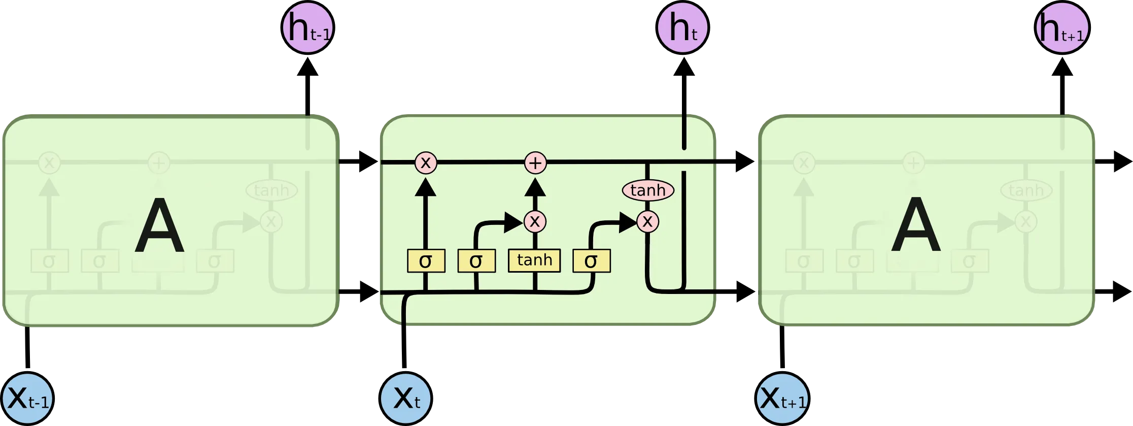
Mathematical Interpretation: How It Stops Vanishing Gradients
In a standard RNN, the gradient flow involves repeated multiplication of the weight matrix:
In contrast, the gradient flow through the cell state in an LSTM is: Here, is the output of the Forget Gate (a value between 0 and 1). If the network learns that the information is important and sets , the gradient flows back through time without being multiplied by weight matrices or activation derivatives. This effectively prevents the gradient from vanishing.
The Metaphor: The Diary
Think of an LSTM as a diary:
- Forget Gate: “Erase the unimportant details from yesterday (like what I had for lunch).”
- Input Gate: “Write down the important new formula I learned today.”
- Output Gate: “Based on what’s in my diary, summarize it to tell my friend what I did.”
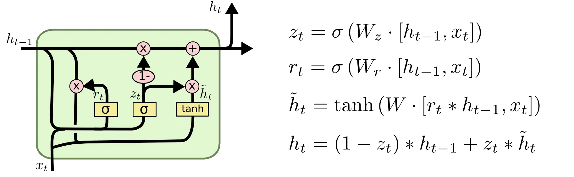
GRU: Gated Recurrent Unit
Proposed by Cho et al. in 2014, the GRU is a streamlined version of the LSTM.
Features
- It combines the forget and input gates into a single update gate.
- It merges the cell state and hidden state, simplifying the architecture.
- With fewer parameters, it is computationally more efficient and often performs on par with LSTMs, especially on smaller datasets.
RNN vs LSTM vs GRU Comparison
| Feature | Standard RNN | LSTM | GRU |
|---|---|---|---|
| Structure | Simple (1 tanh layer) | Complex (4 interacting layers) | Moderate (3 interacting layers) |
| Memory Mechanism | Hidden state only | Cell state + Hidden state | Hidden state only (merged) |
| Gates | None | 3 (Forget, Input, Output) | 2 (Reset, Update) |
| Long-Term Dependencies | Poor (Vanishing Gradients) | Excellent | Very Good |
| Computation Speed | Fast | Slow | Moderate |
| Parameters | Fewest | Most | Moderate |
Quizzes
Quiz 1: Why does the chain rule lead to vanishing gradients in RNNs but not as severely in feed-forward networks?
In RNNs, the same weight matrix is multiplied repeatedly at every time step. In a feed-forward network, different layers have different weight matrices, so the effect of repeated multiplication of the same value is less pronounced, though vanishing gradients still occur in very deep feed-forward networks (which led to ResNets).
Quiz 2: How does the Cell State in an LSTM help prevent vanishing gradients?
The Cell State in an LSTM acts as a conveyor belt with linear interactions (controlled by gates), allowing gradients to flow back through time without being multiplied by shrinking derivatives at every step. This effectively mitigates the vanishing gradient problem.
Quiz 3: What is Gradient Clipping and which problem does it solve?
Gradient Clipping is a technique used to combat exploding gradients. If the norm of the gradient exceeds a certain threshold, it is scaled down to that threshold. This prevents updates from becoming too large and destabilizing training.
Quiz 4: Why are activation functions like ReLU preferred over Sigmoid in deep networks regarding vanishing gradients?
The derivative of the Sigmoid function peaks at 0.25. When multiplying these derivatives in the chain rule, they quickly drive the gradient to zero. The derivative of ReLU is 1 for positive inputs, which does not shrink the gradient when multiplied.
Quiz 5: What is the main difference between LSTM and GRU?
LSTM has three gates (forget, input, output) and maintains a separate cell state and hidden state. GRU is a simpler architecture with only two gates (reset, update) and merges the cell state and hidden state. GRU is computationally more efficient while often achieving similar performance.
Quiz 6: Formulate the necessary condition for the recurrent weight matrix in terms of its spectral radius to prevent exploding gradients, and explain its mathematical justification.
To prevent exploding gradients, a necessary condition is that the spectral radius of the recurrent weight matrix must satisfy . The spectral radius is defined as , where are the eigenvalues of . During Backpropagation Through Time (BPTT), the gradient involves repeated multiplication of the Jacobian . For activation functions like tanh, the derivative satisfies . The norm of the product is bounded by . If the spectral radius , the term will grow exponentially as , causing exploding gradients. Therefore, is a necessary condition for stability.
References
- Hochreiter, S., & Schmidhuber, J. (1997). Long short-term memory. Neural computation, 9(8), 1735-1780.
- Cho, K., et al. (2014). Learning phrase representations using RNN encoder-decoder for statistical machine translation. arXiv:1406.1078.
- Pascanu, R., Mikolov, T., & Bengio, Y. (2013). On the difficulty of training recurrent neural networks. arXiv:1211.5063.