8.4 Transfer Learning & Generalization

In the previous section, we established the economic and physical trade-offs of scaling pre-training compute. However, pre-training a Foundation Model is rarely the final objective; it is merely the initialization phase. The true utility of a model is defined by its ability to transfer its vast, unstructured latent knowledge to specific downstream tasks—whether through Supervised Fine-Tuning (SFT), Reinforcement Learning from Human Feedback (RLHF), or zero-shot application.

This brings us to the science of Generalization. How predictably does pre-training knowledge transfer? What happens to the internal representations of a model when it is forced to adapt to a new distribution? And most critically for the future of AI alignment, how do we transfer intent to a model that is significantly more capable than its human supervisors?

The Physics of Knowledge Transfer

Transfer learning is not a black box; it obeys strict empirical scaling laws. When a pre-trained model is fine-tuned on a downstream dataset, its performance trajectory is fundamentally different from a model trained from scratch.

To quantify this, researchers define a metric called Effective Data Transferred ($D_T$). Suppose we fine-tune a pre-trained model on a downstream dataset of size $D_F$, achieving a specific validation loss $L$. We then ask: How many data points ($D_S$) would a model with the exact same architecture require to achieve that identical loss $L$ if it were trained entirely from scratch?

The effective data transferred is simply the difference: $D_T = D_S - D_F$

Empirical studies [1] reveal that in the low-data regime, $D_T$ scales as a power law with respect to both the model’s parameter count ($N$) and the fine-tuning dataset size ($D_F$): $D_T \approx k \cdot N^\alpha \cdot D_F^\beta$

This equation contains a profound engineering implication. Because $\alpha > 0$, scaling up the parameter count $N$ exponentially increases the amount of effective data transferred. A 100-billion parameter model extracts vastly more generalized utility from 1,000 fine-tuning examples than a 10-billion parameter model does. This is why massive Foundation Models are extraordinary few-shot learners: their scale acts as a physical multiplier on the fine-tuning data.

Grokking: The Delayed Generalization

While scaling laws describe the macroscopic behavior of transfer learning, the microscopic learning dynamics reveal a much stranger phenomenon. For years, the standard assumption was that memorization and generalization were opposing forces, and that generalization improved smoothly as training loss decreased.

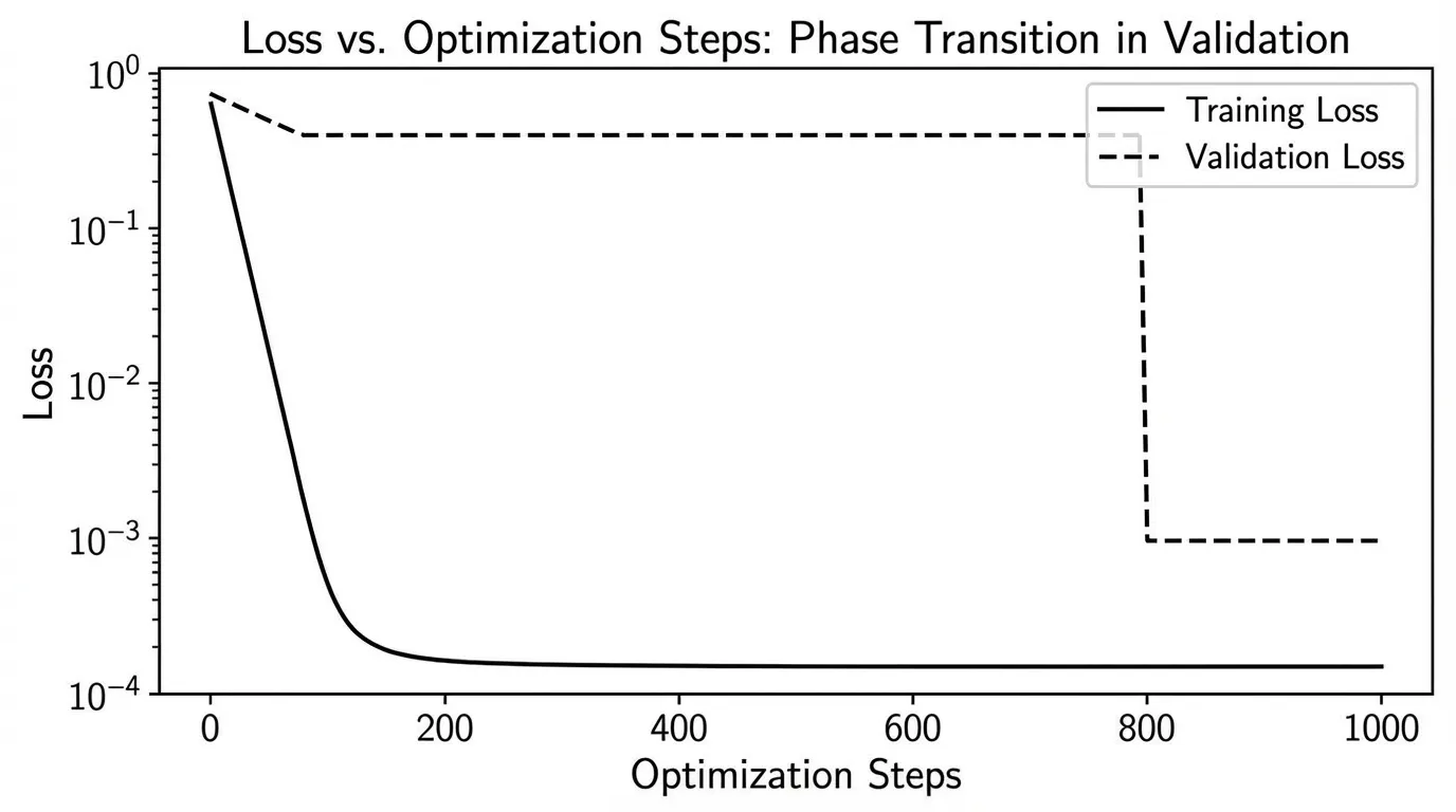
The discovery of Grokking [2] shattered this assumption. In certain regimes, a model will quickly achieve near-zero training loss by perfectly memorizing the dataset, while its validation loss remains extremely high. If training is halted here, the model is deemed overfitted. However, if training continues for thousands of additional steps—long after the training loss has flatlined—the validation loss will suddenly and precipitously drop. The model “groks” the underlying rules of the data.

Recent theoretical breakthroughs [3] have mathematically formalized this delay. Grokking is not magic; it is a norm-driven representational phase transition.

During the initial phase of training, the optimizer finds a “lazy,” high-norm solution that interpolates the training data through brute-force memorization. However, regularizers like weight decay continuously apply a penalty to this high-norm state. Over thousands of steps, the optimizer slowly contracts the weights. Once the weight norm crosses a critical threshold, the memorization circuits collapse, forcing the network to adopt a lower-norm, structured representation that generalizes to unseen data.

The delay before grokking occurs ($T_{grok} - T_{mem}$) follows its own precise scaling law: $T_{grok} - T_{mem} = \Theta\left(\frac{1}{\gamma_{eff}} \log \frac{||\theta_{mem}||^2}{||\theta_{post}||^2}\right)$ Where $\gamma_{eff}$ is the effective contraction rate of the optimizer (e.g., learning rate $\times$ weight decay for SGD), $||\theta_{mem}||$ is the weight norm at the point of memorization, and $||\theta_{post}||$ is the weight norm of the generalizing solution.

This proves that generalization is not always immediate. In complex transfer learning scenarios, the compute spent after apparent convergence is often what crystallizes robust, generalizable circuits.

Weak-to-Strong Generalization

As models scale, we encounter a unique transfer learning bottleneck: The Alignment Problem. Traditionally, we transfer human intent to a model via RLHF or SFT, where humans act as the ground-truth supervisors. But what happens when the model becomes significantly smarter than the human? How do we supervise a system whose outputs we cannot fully comprehend?

To study this empirically, researchers introduced the paradigm of Weak-to-Strong Generalization [4]. The setup is an analogy for superhuman alignment:

1. Take a weak, less capable model (e.g., a 1B parameter model) and train it on a task.
2. Use this weak model to generate noisy, imperfect labels.
3. Fine-tune a strong, highly capable pre-trained model (e.g., a 100B parameter model) using only these weak labels.

The naive assumption is that the strong model will simply imitate the weak model, inheriting all its errors and hallucinated logic. The empirical reality is vastly more optimistic. The strong model consistently outperforms its weak supervisor.

Why? Because the strong model does not learn the task from scratch. It uses the weak labels merely to deduce the format and intent of the task, but it relies on its own robust, pre-trained latent representations to execute the logic. It transfers its pre-existing knowledge to fill in the gaps left by the weak supervisor.

Engineering Confidence

To maximize weak-to-strong generalization, engineers must prevent the strong model from overfitting to the specific errors of the weak supervisor. One highly effective technique is the Auxiliary Confidence Loss.

By adding a penalty that minimizes the entropy of the strong model’s output distribution, we force the model to be highly confident in its predictions. This encourages the strong model to trust its own latent knowledge, allowing it to confidently disagree with the weak supervisor when the supervisor makes an obvious error.

The following PyTorch implementation demonstrates how this loss function is constructed for a classification-based alignment task.

import torch
import torch.nn as nn
import torch.nn.functional as F

class WeakToStrongLoss(nn.Module):
    """
    Implements the Weak-to-Strong generalization objective.
    Forces a strong student model to learn from a weak supervisor's soft labels,
    while maintaining confidence in its own latent representations.
    """
    def __init__(self, confidence_coef: float = 0.2):
        super().__init__()
        # The coefficient controlling how aggressively we push the strong model
        # to be confident in its own predictions.
        self.confidence_coef = confidence_coef

    def forward(
        self, 
        strong_logits: torch.Tensor, 
        weak_soft_labels: torch.Tensor
    ) -> torch.Tensor:
        """
        Args:
            strong_logits: (Batch, Num_Classes) - Raw logits from the strong model.
            weak_soft_labels: (Batch, Num_Classes) - Probability distributions from the weak model.
        """
        # 1. Imitation Loss (KL Divergence)
        # Teaches the strong model the general intent and format of the task
        # based on the weak supervisor's guidance.
        log_probs_strong = F.log_softmax(strong_logits, dim=-1)
        imitation_loss = F.kl_div(
            log_probs_strong, 
            weak_soft_labels, 
            reduction='batchmean'
        )
        
        # 2. Auxiliary Confidence Loss (Entropy Minimization)
        # We minimize the entropy of the strong model's predictions.
        # This prevents the strong model from mimicking the uncertainty of the weak model,
        # encouraging it to "disagree" using its superior pre-trained knowledge.
        probs_strong = F.softmax(strong_logits, dim=-1)
        entropy = -torch.sum(probs_strong * log_probs_strong, dim=-1).mean()
        
        # Total Objective
        total_loss = imitation_loss + self.confidence_coef * entropy
        
        return total_loss

# --- Simulation ---
torch.manual_seed(42)
batch_size, num_classes = 4, 10

# Simulated predictions from a weak supervisor (high uncertainty/entropy)
weak_logits = torch.randn(batch_size, num_classes) * 0.5
weak_soft_labels = F.softmax(weak_logits, dim=-1)

# Simulated raw logits from a strong pre-trained model
strong_logits = torch.randn(batch_size, num_classes) * 2.0

criterion = WeakToStrongLoss(confidence_coef=0.2)
loss = criterion(strong_logits, weak_soft_labels)

print(f"Weak-to-Strong Objective Loss: {loss.item():.4f}")

Generalization is the bridge between raw compute and actual intelligence. Whether we are waiting for a phase transition to grok a complex dataset, or leveraging a model’s latent knowledge to surpass its own supervisor, mastering these transfer dynamics is the key to building autonomous, agentic systems.

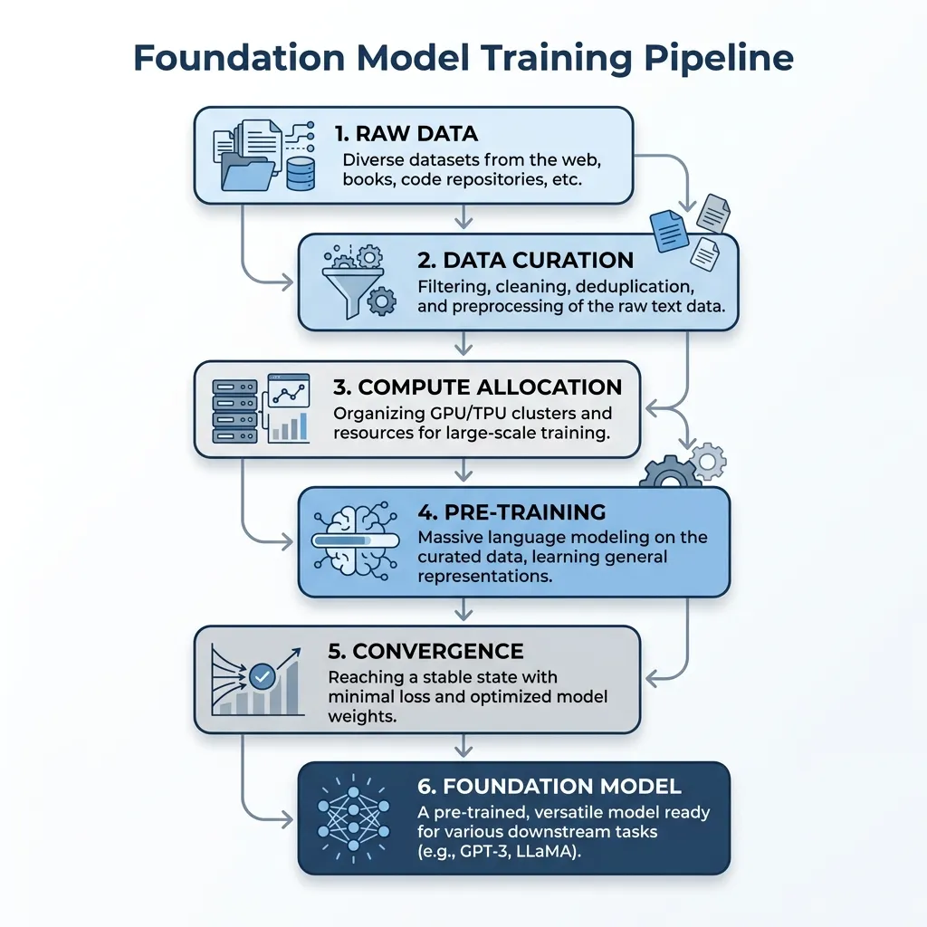
The Foundation Model Training Pipeline: A Synthesis

Having explored Data Engineering (Chapter 6), Architecture (Chapter 7), and Scaling Dynamics (Chapter 8), we can now synthesize the entire training process of a Foundation Model into a unified pipeline.

The journey from raw data to a pre-trained model involves a sequence of carefully orchestrated steps, each governed by the physical and economic principles we have discussed.

The Integrated Workflow

1. Data as the Foundation: The process begins with raw, uncurated data. As seen in Chapter 6, the choice of tokenizer and the rigor of data filtering set the upper bound of the model’s capabilities. High-quality, clean data is non-negotiable.
2. Sizing and Allocation: Before training starts, engineers apply the scaling laws (Chapter 8) to determine the optimal allocation of compute. Whether aiming for Chinchilla optimality or over-training for inference efficiency, this step defines the physical architecture and token budget.
3. The Distributed Crucible: Training a model with billions of parameters requires thousands of GPUs. The model processes tokens, computes loss, and updates weights continuously. Engineers monitor the training loss against the predicted power law curve to detect anomalies.
4. The Result: The output of this massive undertaking is a base Foundation Model—a highly compressed repository of world knowledge, ready to be molded for specific tasks via transfer learning and alignment in the subsequent chapters.

Chapter 8 Summary & Developer Insights

Summary

In this chapter, we explored the physics of scaling foundation models. We started with the Power Law (8.1), which allows us to predict model performance based on compute, data, and parameters. We then looked at Chinchilla Optimality (8.2), which corrected early scaling laws by advocating for equal scaling of parameters and data. However, the economic reality of inference costs led to the era of Over-training (8.3), where models are trained far beyond the Chinchilla-optimal point to create smaller, more efficient models for deployment, despite the risk of catastrophic overtraining and loss of plasticity. Finally, we examined Transfer Learning and Generalization (8.4), understanding how scale acts as a multiplier on fine-tuning data, the phenomenon of grokking, and how strong models can generalize beyond weak supervision.

Developer Insights

• Don’t blindly follow Chinchilla: If you are deploying a model for massive scale, over-training a smaller model is often the right economic choice, even if it wastes training FLOPs.
• Monitor Plasticity: When over-training, monitor the Fisher Information Matrix trace or gradient norms to ensure you don’t push the model into the “brittle” zone where it cannot be instruction-tuned.
• Scale Multiplies Data: Large pre-trained models require significantly less fine-tuning data to achieve the same performance as smaller models. Invest in scale to save on data collection.
• Grokking takes time: If your model seems to be overfitting but the task is algorithmic or highly structured, continue training. Generalization might be just around the corner.

Quizzes

References

1. Hernandez, D., et al. (2021). Scaling Laws for Transfer. arXiv:2102.01293.
2. Power, A., et al. (2022). Grokking: Generalization Beyond Overfitting on Small Algorithmic Datasets. arXiv:2201.02177.
3. Tian, Y. (2026). Why Grokking Takes So Long: A First-Principles Theory of Representational Phase Transitions. arXiv:2603.13331.
4. Burns, C., et al. (2023). Weak-to-Strong Generalization: Eliciting Strong Capabilities With Weak Supervision. arXiv:2312.09390.