14.2 Vector Indexing & DB Solutions
Once documents are converted into high-dimensional vector embeddings, the next challenge is searching through them efficiently. In a production RAG system with millions or billions of vectors, comparing a query vector against every single stored vector (Exact Search) is computationally impossible for real-time responses.
To achieve sub-millisecond latency, we use Approximate Nearest Neighbor (ANN) algorithms. This chapter compares the industry-standard HNSW algorithm with Google’s cutting-edge ScaNN and other approaches, and reviews the commercial Vector DB landscape.
1. The Search Bottleneck: Exact vs. ANN
Exact search (K-Nearest Neighbors or KNN) computes the distance between the query vector and every vector in the database.
- Time Complexity: , where is the number of documents and is the dimension.
- For 1 billion 768-dimensional vectors, one search requires 768 billion operations.
ANN algorithms trade a tiny amount of accuracy (recall) for massive gains in speed, reducing search complexity to or in some cases.
2. HNSW: The King of Vector Indices
HNSW (Hierarchical Navigable Small World) [1] is the most widely used graph-based ANN algorithm. It powers the backends of Pinecone, Milvus, Qdrant, and FAISS.
HNSW builds a multi-layered graph structure inspired by Skip-Lists:
- Layer 0 (Bottom): Contains all vectors in a dense graph.
- Upper Layers: Contain exponentially fewer nodes with links spanning larger distances.
Search starts at the top layer, making large leaps, and drops down to denser layers to fine-tune the result. This reduces complexity to .
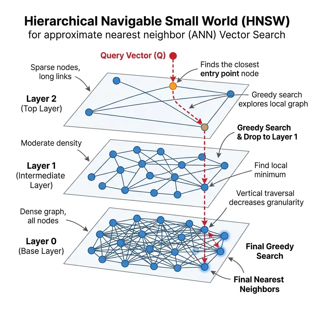
HNSW Routing Visualization
Observe how the query (red) enters at the sparse top layer and drops down to find the nearest neighbors.
HNSW Routing Simulator
Click on an empty space on the graph to create a query (red dot). The search process is visualized as it drops from the upper layer (L2) to the lower layer (L0).
3. Google’s ScaNN: Optimized for MIPS
While HNSW is excellent, Google developed ScaNN (Scalable Nearest Neighbors) [2] specifically for Maximum Inner Product Search (MIPS), which is the operation used when searching by dot product or cosine similarity in embeddings.
The Innovation: Anisotropic Vector Quantization
Traditional quantization (like Product Quantization) tries to minimize the reconstruction error of the vectors themselves (making the quantized vector as close to the original as possible).
ScaNN introduces Anisotropic Quantization. It realizes that for inner product search, we don’t care if the quantized vector is slightly off in length, as long as its direction relative to the query is preserved. ScaNN intentionally introduces errors in the direction orthogonal to the vector to keep the parallel component (the one that determines the dot product) as accurate as possible.
This allows ScaNN to achieve state-of-the-art speed and recall trade-offs, often outperforming HNSW in pure CPU environments for MIPS tasks.
4. Algorithm Comparison Table
Here is a comparison of the major vector indexing algorithms for beginners and experts alike:
| Algorithm | Type | Best For | Pros | Cons |
|---|---|---|---|---|
| HNSW | Graph-based | General purpose, high recall | - State-of-the-art recall/speed balance - Supports dynamic adds/deletes | - High memory consumption - Slow index build time |
| ScaNN | Quantization + Search | MIPS (Dot product), CPU efficiency | - Extremely fast search speed - Low memory footprint | - Complex implementation - Harder to update dynamically |
| IVF (Inverted File) | Clustering | Large scale, low memory | - Fast build time - Low memory | - Lower recall than HNSW - Prone to cluster imbalance |
| Flat (Exact) | Brute Force | Small datasets (<10k) | - 100% accuracy (Recall) - No index build time | - Scales linearly - Too slow for large data |
5. Beyond Vectors: Metadata and Access Control
In a real-world enterprise RAG system, you rarely search by vector similarity alone. Documents have attributes like creation date, author, category, and most importantly, access permissions.
The Need for Metadata
Imagine a company-wide RAG system. A HR document about executive salaries should not be visible to all employees, even if it is the semantically closest match to a query like “What is the salary range for senior roles?”.
To handle this, we attach Metadata to our vectors. Metadata is structured data (JSON-like) associated with each vector, such as:
{
  "doc_id": "HR-2026-001",
  "department": "HR",
  "access_roles": ["admin", "hr_manager"],
  "created_at": "2026-04-01"
}
Metadata Filtering and ANN
The challenge arises when we combine metadata filtering with Approximate Nearest Neighbor (ANN) search. There are two main approaches:
A. Post-Filtering (Naive)
- Perform ANN search to find top similar vectors (e.g., ).
- Filter the results based on metadata (e.g., keep only documents where
access_rolescontainsuser_role).
- Problem: If the top 100 results are all restricted HR documents, and the user is a general employee, post-filtering will return zero results, even if there are relevant public documents further down the list. This is called the “empty result problem.”
B. Pre-Filtering (Harder but Better)
- Filter the database first to keep only vectors the user is allowed to see.
- Perform ANN search on the filtered subset.
- Problem: Pre-filtering can break the graph structure of algorithms like HNSW. If you remove nodes from the graph before searching, you might disconnect paths, leading to poor recall or failed searches.
Modern Solution: Filtered HNSW and Bitmaps
Modern vector databases (like Pinecone, Milvus, and Qdrant) solve this by integrating filtering directly into the ANN search process.
- They maintain bitmaps or inverted indices for metadata.
- During HNSW graph traversal, they check the metadata condition at each step, skipping nodes that don’t match the filter without breaking the traversal path.
Practical Guide for Developers
When implementing Role-Based Access Control (RBAC) in RAG:
- Embed permissions: Always include access control lists (ACLs) in your vector metadata.
- Prefer Pre-filtering: Ensure your chosen Vector DB supports efficient pre-filtering (integrated with ANN) rather than just post-filtering.
- Keep metadata small: Large metadata payloads increase memory consumption and can slow down search. Only store what you need for filtering.
6. Commercial Vector DB & Solutions
When moving from algorithms to infrastructure, developers have several choices for managing vector search:
A. Specialized Vector Databases
- Pinecone: A fully managed, cloud-native vector DB. Great for getting started quickly without managing infrastructure.
- Milvus / Qdrant: Open-source, highly scalable vector databases that can be self-hosted or used as managed services. Optimized for billion-scale searches.
B. Library-based Solutions
- FAISS (Facebook AI Similarity Search): The legendary library by Meta. It is not a database but a set of core algorithms (including HNSW and IVF) written in C++ with Python wrappers. It is the foundation for many other systems.
C. Cloud Provider Solutions
- Google Cloud Vertex AI Vector Search: Formerly known as Matching Engine, it uses ScaNN-like technology under the hood. It offers extreme scale and low latency but can be complex to set up for small projects.
- AWS OpenSearch / Azure AI Search: Traditional search engines that have added vector search capabilities (usually via HNSW plugins). Good if you already use these ecosystems and need hybrid search.
Quizzes
Quiz 1: Why does HNSW consume more memory compared to quantization-based methods like ScaNN or IVF?
HNSW must store the graph structure (pointers/links between nodes) in memory for all layers, in addition to the vectors themselves. Quantization methods compress the vectors and don’t require storing complex graph edges.
Quiz 2: In what scenario would you choose ScaNN over HNSW for a production RAG system?
You would choose ScaNN if your primary constraint is search speed on CPUs and you are using inner product (dot product) as your similarity metric. ScaNN’s anisotropic quantization is specifically optimized for this and can yield higher throughput on standard CPU hardware compared to HNSW.
Quiz 3: Calculate the memory footprint (in bytes) required to store vectors of dimension using Product Quantization (PQ) with sub-vectors and centroids per sub-vector subspace.
PQ decomposes a -dim vector into sub-vectors, each of dimension . Each subspace has centroids, requiring bits ( byte) to store the identifier per sub-vector. Thus, each quantized vector takes exactly bytes. For vectors, storage requires MB. Additionally, the centroids themselves occupy KB. Compared to the unquantized FP32 footprint of GB, PQ delivers a massive memory reduction.
References
- Malkov, Y. A., & Yashunin, D. A. (2016). Efficient and robust approximate nearest neighbor search using Hierarchical Navigable Small World graphs. arXiv:1603.09320.
- Guo, R., et al. (2020). Accelerating Large-Scale Random-Walk Based Search via Anisotropic Vector Quantization. ICML. arXiv:1908.10396.