2.4 CNNs for NLP

While Recurrent Neural Networks (RNNs) were considered the natural choice for sequential data, Convolutional Neural Networks (CNNs), famous for their success in computer vision, were also adapted for Natural Language Processing (NLP).

Motivation: The Need for Speed

The primary motivation for using CNNs in NLP was computational efficiency.

• The RNN Bottleneck: RNNs are inherently sequential. You cannot calculate the state of word 100 without first calculating words 1 through 99. This prevents full parallelization on GPUs.
• The CNN Advantage: Convolutions apply the same operation to different parts of the input simultaneously. This makes them blazingly fast to train.

Before Transformers showed how to achieve both global context and parallelization, CNNs were the go-to choice for fast text processing.

The Metaphor: The Reading Glass

Imagine you are reading a long line of text through a narrow reading glass that only lets you see 3 words at a time.

• You start at the beginning and slide the glass down the line.
• At each stop, you look at the 3 words and recognize a pattern (e.g., “not very good”).
• You write down a score for how strongly that pattern matched what you were looking for.
• By the time you reach the end, you have a list of scores for the whole sentence.
• Max Pooling is like looking at that list and picking the single highest score—the most important pattern you found in the whole sentence.

This is exactly how a 1D convolution works on text.

How 1D Convolutions Work on Text

In computer vision, CNNs use 2D convolutions over pixels. In NLP, we use 1D Convolutions over sequences of word embeddings.

The Mechanism

Imagine a sentence represented as a matrix where each row is a word embedding (e.g., $d=300$).

1. Filter: A filter matrix of size $k \times d$ (where $k$ is the window size, e.g., 3 words) slides down the sentence.
2. Convolution: At each step, it performs an element-wise multiplication and sums the result to produce a single number (a feature).
3. Feature Map: As the filter slides down, it produces a vector of features (a feature map).
4. Pooling: Typically, Max-over-time Pooling is applied, taking the maximum value from the feature map to identify the most important feature in the entire sentence.

This allows the network to capture local patterns (n-grams), such as “not good” or “very fast”.

Breakthrough Architectures

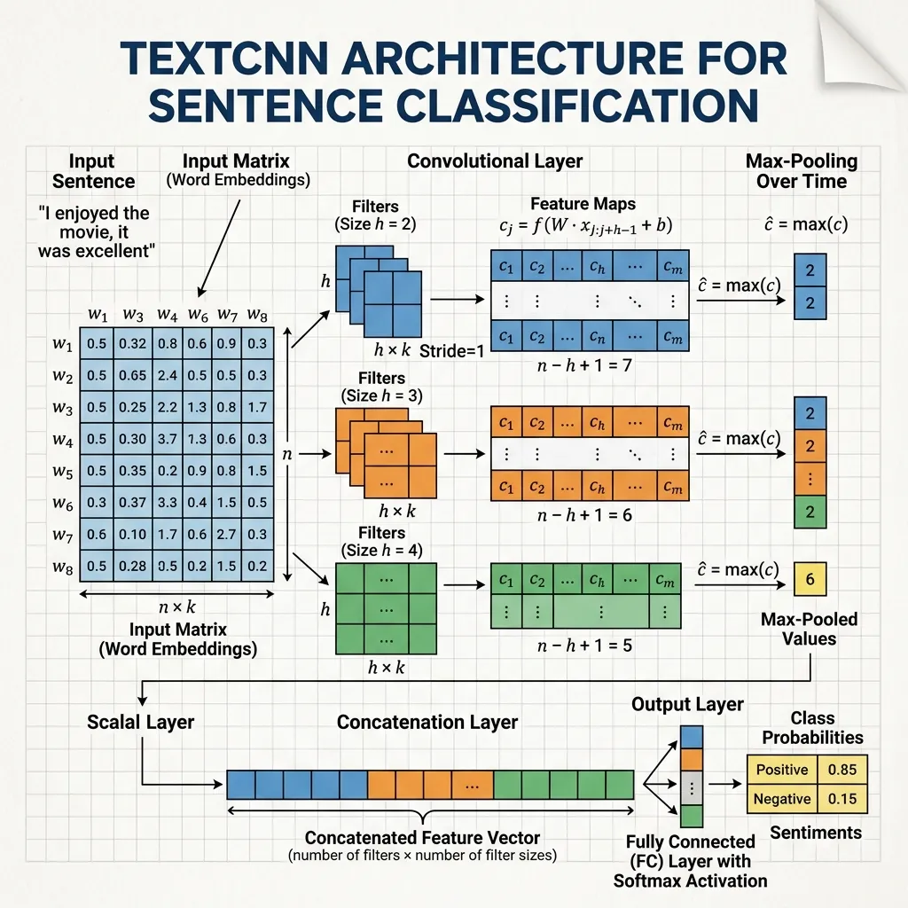
• TextCNN (Kim, 2014) [1]: A simple but effective architecture that uses multiple filter sizes to capture different n-gram lengths, followed by max-pooling. It showed excellent performance on text classification tasks.

Interesting Fact: When Yoon Kim’s TextCNN paper was published, it surprised many researchers. At the time, the dominant view was that “text is a sequence, so we must use RNNs.” However, CNNs were able to capture key word combinations (n-grams) brilliantly, just like they capture local features in images, and most importantly, they were much faster than RNNs.

PyTorch TextCNN

Here is a simplified version of the famous TextCNN architecture (Kim, 2014) [1] in PyTorch, using 1D convolutions for text classification.

import torch
import torch.nn as nn
import torch.nn.functional as F

class TextCNN(nn.Module):
    def __init__(self, vocab_size, embed_dim, num_classes):
        super(TextCNN, self).__init__()
        self.embedding = nn.Embedding(vocab_size, embed_dim)
        
        # 3 different filter sizes: 3, 4, and 5 words
        self.conv1 = nn.Conv1d(in_channels=embed_dim, out_channels=100, kernel_size=3)
        self.conv2 = nn.Conv1d(in_channels=embed_dim, out_channels=100, kernel_size=4)
        self.conv3 = nn.Conv1d(in_channels=embed_dim, out_channels=100, kernel_size=5)
        
        self.fc = nn.Linear(300, num_classes)
        
    def forward(self, x):
        # x shape: (batch_size, seq_len)
        embedded = self.embedding(x) # (batch, seq_len, embed_dim)
        
        # Conv1d expects (batch, channels, seq_len)
        embedded = embedded.transpose(1, 2)
        
        # Apply convolutions and ReLU
        x1 = F.relu(self.conv1(embedded))
        x2 = F.relu(self.conv2(embedded))
        x3 = F.relu(self.conv3(embedded))
        
        # Max-over-time pooling
        x1 = F.max_pool1d(x1, x1.shape[2]).squeeze(2)
        x2 = F.max_pool1d(x2, x2.shape[2]).squeeze(2)
        x3 = F.max_pool1d(x3, x3.shape[2]).squeeze(2)
        
        # Concatenate pool results
        combined = torch.cat((x1, x2, x3), dim=1)
        
        # Fully connected layer
        logits = self.fc(combined)
        return logits

# Example usage
vocab_size = 1000
embed_dim = 50
num_classes = 2
model = TextCNN(vocab_size, embed_dim, num_classes)

# Random input sequence of 10 words
x = torch.randint(0, vocab_size, (1, 10))
logits = model(x)
print("Output Logits Shape:", logits.shape)

Example: Sliding Window Convolution

Visualize how a filter of size 3 slides over a sentence and produces a feature map. Max-pooling picks the highest value.

Looking Ahead: The Need for Global Context

We have seen that CNNs offer speed through parallelization, but they struggle with long-range dependencies compared to RNNs.

• Is it possible to achieve both full parallelization and global context?
• Can we model relationships between all words in a sentence directly, without sequential processing or local windows?
• How does the concept of “Self-Attention” eliminate the need for recurrence and convolution?

These questions lead us to Chapter 3: Transformers, where we will explore the architecture that revolutionized AI by relying entirely on attention.

Quizzes

References

1. Kim, Y. (2014). Convolutional neural networks for sentence classification. arXiv:1408.5882.
2. Recommended Video: 3Blue1Brown: But what is a convolution? A fantastic visual explanation of the mathematical concept of convolution.