3.2 Multi-head Attention (MHA)

While Self-Attention is powerful, applying it once (Single-Head) limits the model’s ability to focus on different types of relationships simultaneously. Multi-Head Attention (MHA) solves this by running multiple attention mechanisms in parallel.

Let’s understand this through a metaphor.

The Metaphor: The Committee of Experts

Imagine you are analyzing a complex legal document.

• Single-Head Attention is like having one general researcher read the document. They might do a good job, but they can only focus on one aspect at a time (e.g., the general meaning).
• Multi-Head Attention is like hiring a committee of experts:
  • Expert 1 focuses on the legal terminology.
  • Expert 2 focuses on the financial implications.
  • Expert 3 focuses on the historical context.

They all read the same document simultaneously but attend to different aspects. In the end, they combine their findings to give a much richer analysis.

In MHA, each “head” learns to attend to different types of relationships (e.g., grammar, coreference, factual links).

Why Multi-Head? (Representation Subspaces)

To understand the benefit of Multi-Head Attention, consider the word “bank”. It can mean a financial institution or the side of a river.

• In a single-head attention mechanism, the model must create a single attention distribution for “bank”. If it needs to capture both the financial context (relating to “money”) and the syntactic context (relating to the preceding article “the”), it has to compromise.
• With Multi-Head Attention, one head can focus on the semantic relationship (bank $\to$ money), while another head can focus on the syntactic relationship (bank $\to$ the).

By projecting the $d_{model}$-dimensional embeddings into $h$ smaller subspaces of dimension $d_k$, each head can specialize in finding specific types of patterns without interference from other patterns. This is analogous to how CNNs use multiple filters to detect different visual features (e.g., edges, textures).

The Mathematics of Multi-Head Attention

Instead of performing a single attention function with $d_{model}$-dimensional keys, values, and queries, MHA linearly projects the queries, keys, and values $h$ times with different, learned linear projections to $d_k, d_k,$ and $d_v$ dimensions, respectively.

$\text{MultiHead}(Q, K, V) = \text{Concat}(\text{head}_1, \dots, \text{head}_h)W^O$

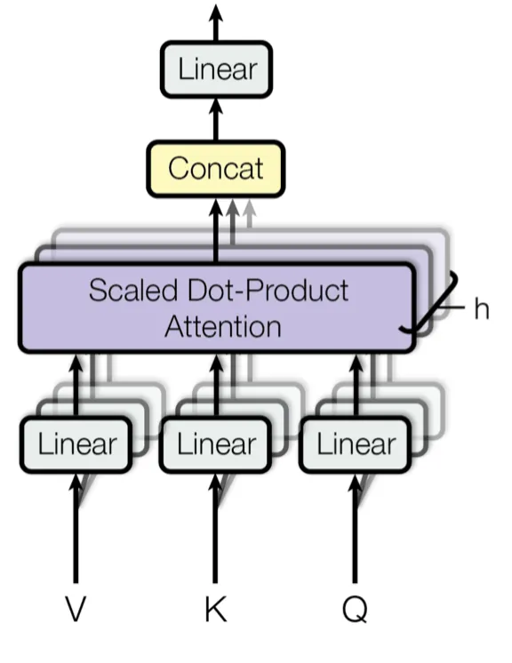
Where: $\text{head}_i = \text{Attention}(QW_i^Q, KW_i^K, VW_i^V)$

And the projections are parameter matrices:

• $W_i^Q \in \mathbb{R}^{d_{model} \times d_k}$
• $W_i^K \in \mathbb{R}^{d_{model} \times d_k}$
• $W_i^V \in \mathbb{R}^{d_{model} \times d_v}$
• $W^O \in \mathbb{R}^{hd_v \times d_{model}}$

Typically, we use $h = 8$ parallel attention heads. For each of these we use $d_k = d_v = d_{model}/h$.

PyTorch Implementation

Here is how you implement Multi-Head Attention in PyTorch. This involves projecting the inputs, splitting them into multiple heads, applying attention, and then concatenating the results.

import torch
import torch.nn as nn
import torch.nn.functional as F

class MultiHeadAttention(nn.Module):
    def __init__(self, d_model, num_heads):
        super(MultiHeadAttention, self).__init__()
        assert d_model % num_heads == 0
        
        self.d_model = d_model
        self.num_heads = num_heads
        self.d_k = d_model // num_heads
        
        # Linear projections for Q, K, V
        self.w_q = nn.Linear(d_model, d_model)
        self.w_k = nn.Linear(d_model, d_model)
        self.w_v = nn.Linear(d_model, d_model)
        
        # Output projection
        self.w_o = nn.Linear(d_model, d_model)
        
    def forward(self, q, k, v, mask=None):
        batch_size = q.size(0)
        
        # 1. Linear projections
        Q = self.w_q(q)
        K = self.w_k(k)
        V = self.w_v(v)
        
        # 2. Split into heads
        # Shape change: (batch, seq_len, d_model) -> (batch, seq_len, num_heads, d_k) -> (batch, num_heads, seq_len, d_k)
        Q = Q.view(batch_size, -1, self.num_heads, self.d_k).transpose(1, 2)
        K = K.view(batch_size, -1, self.num_heads, self.d_k).transpose(1, 2)
        V = V.view(batch_size, -1, self.num_heads, self.d_k).transpose(1, 2)
        
        # 3. Apply Scaled Dot-Product Attention
        scores = torch.matmul(Q, K.transpose(-2, -1)) / (self.d_k ** 0.5)
        if mask is not None:
            scores = scores.masked_fill(mask == 0, -1e9)
        weights = F.softmax(scores, dim=-1)
        attention_output = torch.matmul(weights, V)
        
        # 4. Concatenate heads
        # Shape change: (batch, num_heads, seq_len, d_k) -> (batch, seq_len, num_heads, d_k) -> (batch, seq_len, d_model)
        concat_output = attention_output.transpose(1, 2).contiguous().view(batch_size, -1, self.d_model)
        
        # 5. Output projection
        output = self.w_o(concat_output)
        
        return output, weights

# Example usage
mha = MultiHeadAttention(d_model=64, num_heads=8)
x = torch.randn(2, 10, 64) # Batch of 2, sequence length 10, d_model 64
output, weights = mha(x, x, x)
print("Output Shape:", output.shape)
print("Attention Weights Shape:", weights.shape)

Example: Diverse Perspectives

Visualize how two different heads might attend to the sentence “The bank was full of money.”

• Head 1 might learn to associate “bank” with “money” (financial context).
• Head 2 might learn to associate “bank” with “river” (if the context were different, but here it’s money).

Select a head to see its simulated attention pattern for the word “bank”.

Quizzes

References

1. Vaswani, A., et al. (2017). Attention is all you need. In Advances in neural information processing systems (pp. 5998-6008). arXiv:1706.03762.