14.1 From Lexical to Semantic Search

In Chapter 13, we explored how to make Large Language Models smaller and faster through quantization and compression. While these techniques allow us to run powerful models on limited hardware, they do not solve a fundamental limitation of all foundation models: static parametric knowledge.

A model’s knowledge is frozen at the point of its training cut-off. It cannot answer questions about events after that date, nor can it access your private data or proprietary documents.

To bridge this gap, we need Retrieval-Augmented Generation (RAG). Instead of trying to bake all the world’s knowledge into the model’s parameters (which is expensive and leads to hallucinations), RAG allows the model to dynamically search an external database for relevant information at query time.

This chapter marks the transition from optimizing the model itself to building the retrieval infrastructure around it. We start by understanding the fundamental shift from keyword matching to meaning matching.

In the early days of information retrieval, finding relevant documents relied almost entirely on Lexical Search (keyword search). While this approach powered the first generation of search engines and database queries, it suffers from fundamental limitations when applied to modern RAG systems. To build systems that truly understand user intent, we must transition from searching for words to searching for meaning.

This sub-chapter explains why vector embeddings are necessary, compares lexical and semantic search with an interactive demonstration, and explores advanced chunking strategies to prepare data for retrieval.

1. The Limits of Keyword Search

Lexical search operates on the principle of exact or fuzzy string matching. Algorithms like TF-IDF and BM25 count term frequencies and inverse document frequencies to rank documents. While highly optimized and fast, they fail in several critical scenarios:

A. The Synonym Problem (Vocabulary Mismatch)

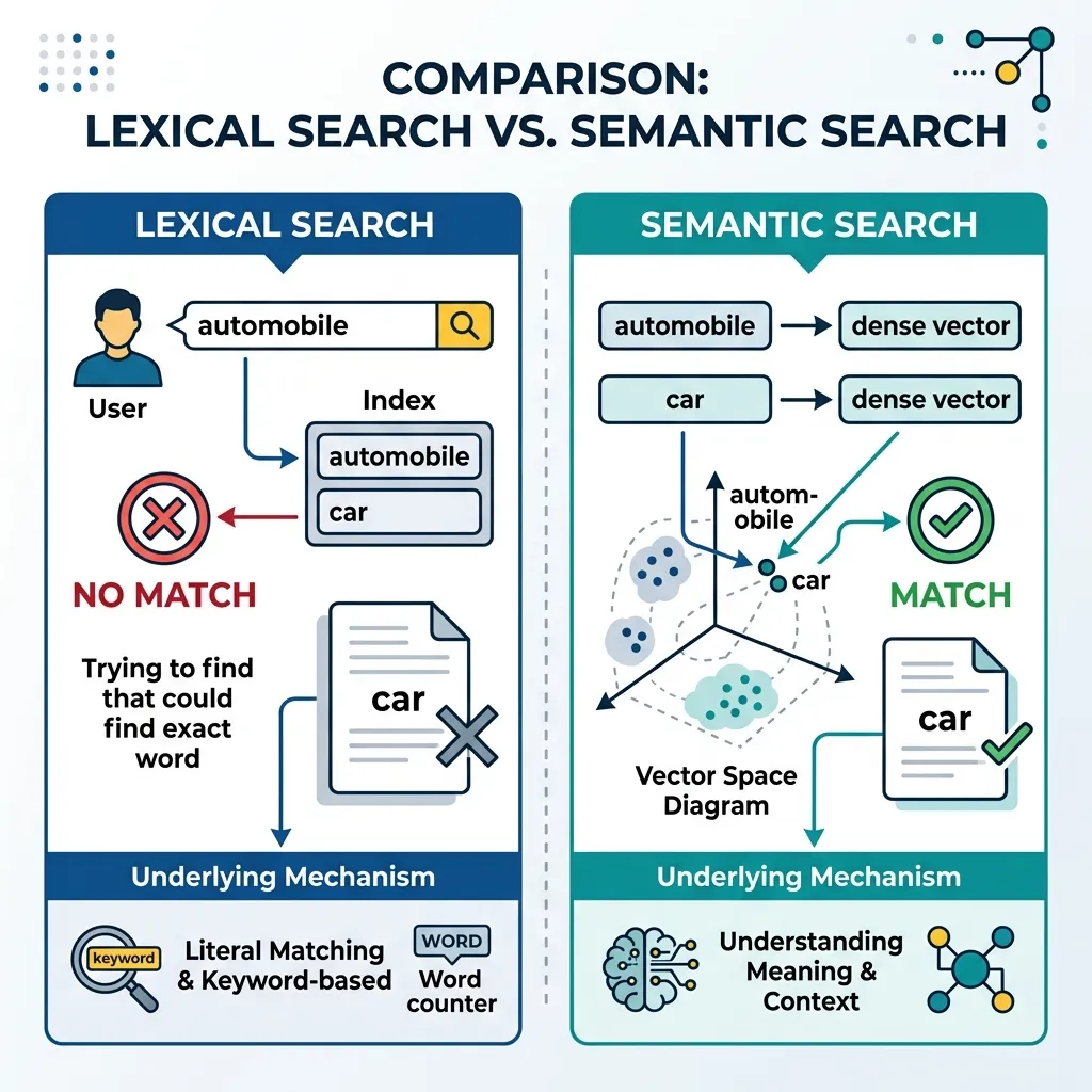
If a user searches for “automobile” but the source document uses the word “car,” a strict lexical search will fail to connect them despite their identical meaning. This is known as vocabulary mismatch.

B. Polysemy (Context Blindness)

The word “bank” can mean a financial institution or the side of a river. Lexical search cannot distinguish between these meanings without additional context words, often leading to irrelevant results.

C. Cross-Lingual Limitations

Keyword search is strictly bound to the language of the query. A search in English cannot retrieve a relevant document written in Korean or Spanish, even if the content is exactly what the user needs.

D. The Solution: Vector Embeddings

To overcome these limits, we represent text as high-dimensional vectors where geometric distance corresponds to semantic similarity. An embedding model (like a fine-tuned BERT or a modern contrastive model) maps the concept of “automobile” and “car” to nearby points in the vector space, solving the synonym problem and enabling cross-lingual retrieval.

2. Interactive Concept: Lexical vs. Semantic Search

To understand the trade-offs, let’s look at a conceptual diagram and then interact with the visualizer below. We have a small database of documents covering various topics.

Try searching for concepts not explicitly mentioned in the text (e.g., searching for “puppy” when the text says “young dog”) to see how semantic search shines, and observe where keyword search might still be necessary (e.g., for specific product codes).

The Keyword Stronghold: Precision on Specifics

As demonstrated above, semantic search is not a silver bullet. It tends to “blur” highly specific tokens like serial numbers, part codes, or rare proper nouns into general categories. For example, searching for Err-404 might retrieve documents about “web errors” in general rather than the specific log entry containing that exact string.

This is why enterprise RAG systems almost always employ Hybrid Search (combining both methods), which we will cover in sub-chapter 14.3.

3. Advanced Chunking Strategies

Before we can embed text and store it in a vector database, we must break large documents into smaller, coherent pieces called chunks. The way we chunk data dramatically impacts retrieval quality.

A. Naive (Fixed-Size) Chunking

The simplest approach is to split text into chunks of a fixed number of tokens (e.g., 256 tokens) with a small overlap (e.g., 20 tokens) to prevent cutting sentences in half.

• Pros: Simple to implement, predictable compute cost.
• Cons: Often breaks semantic coherence, splitting a paragraph or a list across two chunks, leading to loss of context.

B. Hierarchical Chunking

Instead of treating all chunks equally, hierarchical chunking maintains the document structure.

1. Summary Chunk: A high-level summary of a large section (e.g., a whole chapter).
2. Detail Chunks: Smaller chunks containing the actual text of that section.

• Retrieval can first search the summary chunks to identify the relevant section, and then narrow down to the detail chunks, reducing search space and improving precision.

C. Parent-Child (Small-to-Large) Chunking

This is one of the most effective strategies for RAG.

• The Problem: Small chunks are better for precise vector search (less noise), but large chunks provide better context for the LLM to generate an answer.
• The Solution: We break the document into small child chunks (e.g., 50 tokens) for retrieval. Each child chunk is linked to a larger parent chunk (e.g., 500 tokens). When the system retrieves a highly relevant child chunk, it actually feeds the corresponding parent chunk to the LLM.

4. The Mathematics of Semantic Space (InfoNCE and Matryoshka)

To understand how models create these semantic spaces, we must look at how they are trained. Modern dense retrievers are typically trained using Contrastive Learning.

Contrastive Learning and InfoNCE Loss

The goal of contrastive learning is to learn an embedding space where similar items are close together and dissimilar items are far apart. In RAG, this means a query $q_i$ should be close to its relevant document $d_i^+$ (positive sample) and far from other non-relevant documents $d_j$ (negative samples).

The standard loss function for this is InfoNCE (Information Noise Contrastive Estimation):

$\mathcal{L}_{InfoNCE} = -\frac{1}{N} \sum_{i=1}^{N} \log \frac{\exp(\text{sim}(q_i, d_i^+) / \tau)}{\sum_{j=1}^{N} \exp(\text{sim}(q_i, d_j) / \tau)}$

Here:

• $\text{sim}(a, b)$ is a similarity metric, usually dot product or cosine similarity.
• $\tau$ is a temperature parameter that scales the distribution.
• The formula essentially calculates the probability that the positive document is correctly identified among a set of negative documents, framed as a multi-class classification problem.

Matryoshka Representation Learning (MRL)

In large-scale systems, storing high-dimensional vectors (e.g., 768 or 1536 dimensions) for billions of documents becomes extremely expensive in terms of memory and search latency.

Matryoshka Representation Learning (MRL) [1] solves this by training the model to pack information into the early dimensions of the vector. Inspired by Russian nesting dolls (Matryoshka), MRL ensures that the first $K$ dimensions (e.g., 64, 128, 256) are independently capable of high-quality retrieval.

Developers can truncate a 768-dimensional vector to just 128 dimensions. This reduces storage and compute costs by $6\times$ while retaining up to 95% of the original retrieval performance. This “elastic” embedding capability is crucial for optimizing cost-performance trade-offs in production RAG pipelines.

Quizzes

References

1. Kusupati, A., et al. (2022). Matryoshka Representation Learning. arXiv:2205.13147.