8.2 Chinchilla Optimality: The 20-Token Rule

Kaplan’s scaling laws proved that AI performance was predictable, triggering an industry-wide arms race to build the largest possible models. By 2021, the prevailing wisdom was that parameter count ($N$) was the primary driver of intelligence. If you secured a massive GPU cluster, the mathematically “correct” thing to do was to instantiate an enormous model and train it on whatever data you had available.

This era produced behemoths like OpenAI’s GPT-3 (175B parameters) and DeepMind’s Gopher (280B parameters). According to Kaplan’s formulas, if you increased your compute budget by 10x, you should allocate that compute by increasing the model size by roughly 5x, and the dataset size by only 2x.

In 2022, DeepMind published a paper that fundamentally corrected this trajectory. Hoffmann et al. [1] proved that the industry had been building models that were entirely too large for the amount of data they were trained on. This course correction is now known as Chinchilla Optimality.

The Flaw in the Original Power Law

How did Kaplan et al. get it wrong? The error lay in the hyperparameter tuning of their small-scale experiments, specifically the learning rate schedule.

In the original OpenAI experiments, the researchers used a fixed cosine learning rate decay schedule across models of different sizes. However, larger models trained on fewer tokens reach the end of their training runs faster. Because the learning rate schedule was not properly stretched or compressed to match the exact number of training steps (tokens) for each specific model size, the smaller models were systematically disadvantaged in the empirical data.

Hoffmann’s team at DeepMind re-ran hundreds of scaling experiments, meticulously tuning the learning rate schedule to decay exactly to zero at the final training token for every individual run.

The Revised Scaling Equations

With the corrected methodology, Hoffmann et al. discovered that model size ($N$) and data size ($D$) should not scale asymmetrically. To achieve the lowest possible loss for a given compute budget ($C$), model size and training tokens must scale in equal proportions.

Given the compute approximation for Transformers: $C \approx 6ND$

The Chinchilla optimal allocation dictates: $N_{opt} \propto C^{0.5}$ $D_{opt} \propto C^{0.5}$

Empirically, this translates to a simple, golden rule of thumb: For every 1 parameter in a model, you should train it on approximately 20 tokens of data.

The Gopher vs. Chinchilla Case Study

To prove their revised scaling laws, DeepMind trained a new model named Chinchilla. They gave it the exact same compute budget that was used to train their previous flagship model, Gopher.

• Gopher (Pre-Chinchilla): 280 Billion parameters, trained on 300 Billion tokens. (Ratio: ~1.1 tokens per parameter).
• Chinchilla (Compute-Optimal): 70 Billion parameters, trained on 1.4 Trillion tokens. (Ratio: 20 tokens per parameter).

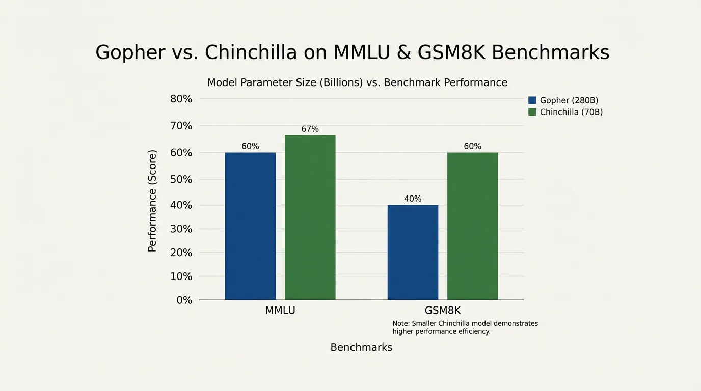
Despite being four times smaller, Chinchilla had seen nearly five times as much data. Because it was compute-optimal, Chinchilla significantly outperformed Gopher on virtually every downstream benchmark.

This realization sent shockwaves through the industry. It meant that a 175B parameter model like GPT-3, which was trained on roughly 300B tokens, was massively undertrained. To be compute-optimal, a 175B model requires 3.5 Trillion tokens—a dataset size that did not exist at the time.

Engineering the Compute Allocation

For Foundation Model engineers, the Chinchilla ratio is the starting point for any cluster allocation. Before writing a single line of model architecture, engineers must balance the target parameter count against the available high-quality data and the physical constraints of their hardware.

Architectural Sizing with PyTorch

Estimating parameters isn’t just about picking a number; it requires defining a physical Transformer architecture (layers, heads, embedding dimensions) that yields the target parameter count, and then calculating the Chinchilla-optimal token count.

The following Python code demonstrates how engineers map architectural hyperparameters to compute requirements using the Chinchilla framework.

import torch

class ComputeEstimator:
    def __init__(self, vocab_size: int = 32000):
        self.vocab_size = vocab_size

    def estimate_transformer_params(self, d_model: int, n_layers: int, n_heads: int) -> int:
        """
        Estimates the non-embedding parameter count of a standard Decoder-only Transformer.
        """
        # Attention parameters: W_q, W_k, W_v, W_o (each is d_model x d_model)
        attn_params_per_layer = 4 * (d_model ** 2)
        
        # FFN parameters: typically up-projects to 4 * d_model, then down-projects
        # W_1: d_model x (4 * d_model), W_2: (4 * d_model) x d_model
        ffn_params_per_layer = 2 * (d_model * (4 * d_model))
        
        # LayerNorms (2 per layer, scale and bias)
        ln_params_per_layer = 4 * d_model
        
        params_per_layer = attn_params_per_layer + ffn_params_per_layer + ln_params_per_layer
        total_non_embedding_params = n_layers * params_per_layer
        
        return total_non_embedding_params

    def chinchilla_prescription(self, d_model: int, n_layers: int, n_heads: int):
        """
        Calculates the optimal dataset size and required compute.
        """
        N = self.estimate_transformer_params(d_model, n_layers, n_heads)
        
        # Chinchilla Rule: 20 tokens per parameter
        D = 20 * N
        
        # Total Compute: C = 6 * N * D
        C = 6 * N * D
        
        print(f"Architecture: {n_layers} Layers, {d_model} d_model, {n_heads} Heads")
        print(f"Non-Embedding Parameters (N): {N / 1e9:.2f} Billion")
        print(f"Optimal Dataset Size (D):     {D / 1e9:.2f} Billion Tokens")
        print(f"Required Compute (C):         {C / 1e21:.2f} ZettaFLOPs\n")

# Example: Sizing a Llama-1 7B style architecture
estimator = ComputeEstimator(vocab_size=32000)

# Llama 7B architecture approximations
estimator.chinchilla_prescription(d_model=4096, n_layers=32, n_heads=32)

# Scaling up to a GPT-3 175B style architecture
estimator.chinchilla_prescription(d_model=12288, n_layers=96, n_heads=96)

Beyond Chinchilla: The Era of Over-training

While Chinchilla optimality defines the most efficient use of training compute, the modern AI landscape has largely abandoned it.

If you are a research lab trying to achieve the lowest possible loss for a fixed $10M budget, you follow Chinchilla. But if you are deploying a model to millions of users, training compute is a one-time fixed cost, while inference compute is a recurring, unbounded operational cost.

This economic reality birthed the era of Over-training (or Inference-Optimal scaling).

Meta’s Llama 3 (8B) is the prime example [2]. According to Chinchilla, an 8B parameter model requires roughly 160 Billion tokens to be compute-optimal. Meta trained Llama 3 8B on 15 Trillion tokens—nearly 100 times the Chinchilla recommendation (a ratio of ~1875:1).

Why? Because pushing an 8B model far past its training-optimal point forces the small network to compress immense amounts of knowledge. The result is a model that rivals the intelligence of a 70B model, but is small enough to run locally on a MacBook or be served incredibly cheaply in the cloud. We sacrifice training efficiency to achieve inference efficiency.

Chinchilla optimality remains the baseline physics of model scaling, but engineering is about trade-offs. Today, the constraint is no longer just “compute,” but the availability of high-quality data to fuel the over-training paradigm.

Quizzes

References

1. Hoffmann, J., et al. (2022). Training Compute-Optimal Large Language Models. arXiv:2203.15556.
2. Touvron, H., et al. (2024). The Llama 3 Herd of Models. arXiv:2407.21783.