2.1 Markov Chains to RNNs

Before the revolution of Transformers, modeling sequential data like natural language required architectures designed to handle temporal dependencies. This journey started with simple statistical models and led to the development of Recurrent Neural Networks (RNNs).

Motivation: The Arrow of Time in Data

Most traditional machine learning models assume that data points are independent and identically distributed (i.i.d.). However, language is inherently sequential. The meaning of a word depends on what came before it.

Context Matters: “I am going to the bank” (river bank or financial bank?) depends on the surrounding words.
Variable Length: Sentences can be 3 words or 100 words long. We need architectures that can handle this flexibility.

Understanding how we moved from simple statistics to neural memory is crucial for grasping why Transformers were necessary.

The Metaphor: The Conveyor Belt with Memory

Imagine you are a worker at a conveyor belt, inspecting objects passing by.

The Markov Approach is like having a goldfish memory. You look at the current object and maybe the one right before it. You make a decision based only on that tiny window. If a red ball comes after a green ball, you perform an action. You have no idea what passed by 5 minutes ago.
The RNN Approach is like having a notebook. As each object passes, you look at it, read your notebook (previous hidden state), make a decision, and then update your notebook with new notes. Even if the red ball appeared 10 objects ago, a note about it might still be in your notebook, influencing your current decision.

RNNs introduced this “notebook” (hidden state) to maintain memory across time.

Markov Chains: The Simplest Sequence Models

A Markov Chain is a stochastic model describing a sequence of possible events in which the probability of each event depends only on the state attained in the previous event.

A Piece of History: When the Russian mathematician Andrey Markov first introduced this concept in 1913, his application was to analyze the sequence of letters in Alexander Pushkin’s poem Eugene Onegin. He manually counted 20,000 letters to show that the probability of a vowel following another vowel was different from following a consonant, proving that letters in language are not independent. This became an early statistical precursor to language modeling.

The Markov Property

Mathematically, a sequence of random variables $X_1, X_2, X_3, \dots$ has the Markov property if: $P(X_{n+1} = x | X_1 = x_1, X_2 = x_2, \dots, X_n = x_n) = P(X_{n+1} = x | X_n = x_n)$

In NLP, an $n$ -gram model is a type of Markov chain. A bigram model predicts the next word based only on the previous word.

The Limitation: Natural language is not Markovian. Understanding a sentence often requires memory of words that appeared much earlier. Markov chains fail to capture long-range dependencies.

Why Markov Models Still Matter

Even though $n$ -gram models are too limited for modern language modeling, they teach two important lessons that never went away.

First, they make the sequence problem explicit: prediction quality depends on what information from the past the model is allowed to use. Second, they show the engineering trade-off between context size and data sparsity. If we increase the Markov order from bigrams to 5-grams, the model can use more context, but the number of possible histories explodes and most of them are rarely observed. In practice, early language modeling spent enormous effort on smoothing, backoff, and counting tricks because larger context windows created brittle statistics.

RNNs were attractive because they replaced this manually designed fixed window with a learned hidden state. Instead of storing counts for every possible history, the model learned a compressed representation of history.

Recurrent Neural Networks (RNNs): Adding Memory

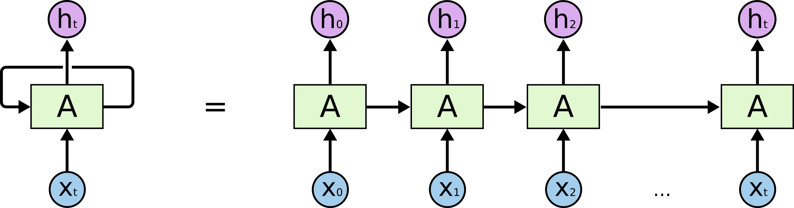
To capture long-term dependencies, Recurrent Neural Networks (RNNs) were developed. Unlike standard feed-forward networks, RNNs have connections that loop back, allowing information to persist.

RNN Unrolled

Source: colah’s blog

The Mechanism

At each time step $t$ , the RNN takes an input vector $\mathbf{x}_t$ and the hidden state from the previous time step $\mathbf{h}_{t-1}$ . It computes the new hidden state $\mathbf{h}_t$ and the output $\mathbf{y}_t$ :

$\mathbf{h}_t = \sigma(\mathbf{W}_{hh}\mathbf{h}_{t-1} + \mathbf{W}_{xh}\mathbf{x}_t + \mathbf{b}_h)$ $\mathbf{y}_t = \text{softmax}(\mathbf{W}_{hy}\mathbf{h}_t + \mathbf{b}_y)$

Where $\mathbf{W}$ are weight matrices and $\sigma$ is an activation function (typically tanh in a vanilla RNN).

The hidden state $\mathbf{h}_t$ acts as the network’s memory, accumulating information over time.

Training Reality: Unrolling Through Time

The conceptual diagram of an RNN often hides the operational detail that makes training difficult: the same cell is reused over and over across the entire sequence. During training we unroll the network through time, turning one recurrent cell into a very deep computation graph with shared weights.

That has two immediate consequences:

Teacher forcing: during training, the model is often fed the true previous token rather than its own prediction so the optimization problem stays stable.
Backpropagation Through Time (BPTT): gradients must flow through every unrolled step, so the effective depth of the network grows with sequence length.

This is the key reason RNNs were such an important milestone but also such a frustrating one in practice. They gave us a way to model variable-length context, but they did so with a sequential computation graph that was hard to parallelize and numerically fragile over long horizons. The next sub-chapters on LSTMs, GRUs, and eventually attention can be read as attempts to keep the good part, learned sequence memory, while removing the bad part, unstable long-range credit assignment.

PyTorch RNN

Let’s see how a basic RNN cell is implemented in PyTorch and how we loop over a sequence.

import torch
import torch.nn as nn

class SimpleRNN(nn.Module):
    def __init__(self, input_size, hidden_size, output_size):
        super(SimpleRNN, self).__init__()
        self.hidden_size = hidden_size
        
        # RNN Cell operations
        self.i2h = nn.Linear(input_size + hidden_size, hidden_size)
        self.i2o = nn.Linear(input_size + hidden_size, output_size)
        self.tanh = nn.Tanh()
        self.softmax = nn.LogSoftmax(dim=1)

    def forward(self, input, hidden):
        # Concatenate input and hidden state
        combined = torch.cat((input, hidden), 1)
        hidden = self.tanh(self.i2h(combined))
        output = self.i2o(combined)
        output = self.softmax(output)
        return output, hidden

    def initHidden(self):
        return torch.zeros(1, self.hidden_size)

# Example usage
input_size = 5  # e.g., one-hot vector size
hidden_size = 10
output_size = 5

rnn = SimpleRNN(input_size, hidden_size, output_size)

# Simulate a sequence of 3 words
seq_len = 3
hidden = rnn.initHidden()

# Random input sequence (seq_len, batch_size, input_size)
sequence = torch.randn(seq_len, 1, input_size)

for i in range(seq_len):
    output, hidden = rnn(sequence[i], hidden)
    print(f"Step {i+1} Output shape:", output.shape)
    print(f"Step {i+1} Hidden shape:", hidden.shape)

Example: The Fading Memory of RNN

Visualize how the hidden state changes as words are processed. Notice how early words have less influence as more words are added (Vanishing Gradient problem in disguise).

Sentence: "The cat sat on the mat."

Hidden State Memory Breakdown:

100%

The

Quizzes

Quiz 1: Why are n-gram models considered Markovian?

Because an n-gram model predicts the next token based only on a fixed window of $n-1$ previous tokens. It assumes that history beyond that window does not affect the future, which is the core assumption of a Markov model.

Quiz 2: What is the purpose of the hidden state in an RNN?

The hidden state acts as the network’s memory. It carries information from previous time steps and combines it with the current input to produce the current hidden state and output. This allows the network to process sequential data and capture temporal dependencies.

Quiz 3: Can a standard RNN process sequences of infinite length?

In theory, yes, because the same operation is applied at each time step recursively. In practice, no, because the memory fades quickly (vanishing gradients) and numerical instabilities prevent learning over very long sequences.

Quiz 4: What is the main difference between a bigram model and an RNN?

A bigram model (1st order Markov chain) only looks at the immediately preceding word to predict the next one. An RNN can potentially retain information from all previous words in the sequence via its hidden state, although in practice it struggles with very long-range dependencies.

Quiz 5: Why is parallelization difficult in RNNs compared to CNNs or Transformers?

Parallelization is difficult in RNNs because the computation at time step $t$ depends on the hidden state from time step $t-1$ . This sequential dependency prevents processing all elements of the sequence at once, unlike CNNs or Transformers where operations can be parallelized across the sequence length.

Quiz 6: Mathematically derive the gradient

\frac{\partial L_t}{\partial \mathbf{h}_k}

for

k \ll t

in a recurrent neural network using Backpropagation Through Time (BPTT), and explain how the term

\prod_{j=k+1}^t \frac{\partial \mathbf{h}_j}{\partial \mathbf{h}_{j-1}}

causes vanishing gradients.

The hidden state update is $\mathbf{h}_j = \tanh(\mathbf{W}_{hh}\mathbf{h}_{j-1} + \mathbf{W}_{xh}\mathbf{x}_j + \mathbf{b}_h)$ . By the chain rule, the gradient of the loss $L_t$ at step $t$ with respect to hidden state $\mathbf{h}_k$ is: $\frac{\partial L_t}{\partial \mathbf{h}_k} = \frac{\partial L_t}{\partial \mathbf{h}_t} \frac{\partial \mathbf{h}_t}{\partial \mathbf{h}_k} = \frac{\partial L_t}{\partial \mathbf{h}_t} \prod_{j=k+1}^t \frac{\partial \mathbf{h}_j}{\partial \mathbf{h}_{j-1}}$ . The Jacobian matrix is $\frac{\partial \mathbf{h}_j}{\partial \mathbf{h}_{j-1}} = \text{diag}(1 - \tanh^2(\mathbf{W}_{hh}\mathbf{h}_{j-1} + \dots)) \mathbf{W}_{hh}^T$ . If the weights are small or the activation saturates (value close to $\pm 1$ ), the absolute value of the eigenvalues of the Jacobian is less than $1$ . As $t - k$ becomes large, the product $\prod_{j=k+1}^t \frac{\partial \mathbf{h}_j}{\partial \mathbf{h}_{j-1}}$ geometrically approaches zero, causing the gradient to vanish.

References

Rosenblatt, F. (1958). The perceptron: a probabilistic model for information storage and organization in the brain. Psychological review, 65(6), 386.
Rumelhart, D. E., Hinton, G. E., & Williams, R. J. (1986). Learning representations by back-propagating errors. Nature, 323(6088), 533-536.
Lipton, Z. C., Berkowitz, J., & Elkan, C. (2015). A Critical Review of Recurrent Neural Networks for Sequence Learning. arXiv:1506.00019.
Recommended Video: StatQuest: Recurrent Neural Networks (RNNs) A great visual explanation of how RNNs work.