3.5 Complexity Analysis
To understand why Transformers replaced RNNs and CNNs as the foundation of modern AI, we must analyze their computational complexity. This analysis reveals the trade-offs between computation, parallelization, and the ability to model long-range dependencies.
Motivation: The Cost of Scale
As we move towards processing entire books or long videos, the length of the sequence () grows.
- Computational Complexity: How many operations does it take to process a sequence?
- Parallelization: Can we compute everything at once, or must we wait for step-by-step results?
- Path Length: How many steps must a signal travel between two distant words?
Analyzing these factors explains why Transformers scale better on GPUs but struggle with extremely long context windows.
The Metaphor: Finding a Book in a Library
Imagine you are looking for a specific reference in a library.
- RNN Approach is like walking down the aisles. You start at the first shelf and look at each book one by one. If the sequence is long, it takes a long time. You cannot start looking at shelf 10 until you’ve walked past shelves 1-9. This is sequential operations.
- Transformer Approach is like having a teleportation device. You can compare your query against all books in the library simultaneously. However, to do this, you must build a massive index comparing every book to every other book. This requires a lot of initial work ( operations), but once done, you can find connections instantly in 1 step.
The Complexity Comparison
The authors of “Attention Is All You Need” [1] provided a comparison of self-attention against recurrent and convolutional layers.
| Layer Type | Complexity per Layer | Sequential Operations | Maximum Path Length |
|---|---|---|---|
| Self-Attention | |||
| Recurrent | |||
| Convolutional |
Where:
- is the sequence length.
- is the representation dimension.
- is the kernel size of convolutions.
Analysis of the Trade-offs
-
Complexity per Layer:
- Self-Attention is . It is quadratic in sequence length . When (which was typical in 2017), self-attention is cheaper than recurrent layers. However, as context windows grow (e.g., ), becomes the dominant cost.
- Recurrent is . It is linear in but quadratic in .
-
Sequential Operations:
- Self-Attention is . All operations can be performed in parallel, maximizing GPU utilization.
- Recurrent is . It requires sequential steps, preventing parallelization across time.
-
Maximum Path Length:
- Self-Attention is . Any two positions can interact directly in a single step.
- Recurrent is . A signal must travel through hidden states to connect the first and last token, leading to vanishing gradients.
- Convolutional is with dilated convolutions, which is better than RNNs but worse than Transformers.
Derivation of Complexities
To truly understand these numbers, let’s derive them from the matrix operations involved.
1. Self-Attention:
Recall the formula: . Let’s assume for simplicity.
- Operation: We multiply matrix () by (). To compute one element of the result, we do a dot product of two -dimensional vectors (cost ). Since the result is an matrix, we do this times. Total cost: .
- Softmax Operation: Applied to each row of the matrix. Cost: .
- Multiplying by : We multiply the attention weights matrix () by (). To compute one element of the result, we do a dot product of an -dimensional row and an -dimensional column (cost ). The result is . Total cost: .
- Combining these, the dominant term is .
2. Recurrent (RNN):
In an RNN, the hidden state at step is computed as .
- Assume the hidden state and input both have dimension .
- The matrix-vector multiplication involves a matrix and a vector. This takes operations.
- We must repeat this sequentially for all tokens in the sequence.
- Total cost: .
Memory Complexity Simulation
Let’s look at how the memory required for the self-attention matrix grows quadratically with sequence length. This PyTorch-based simulation estimates the memory needed for the attention scores matrix.
import torch

def estimate_attention_memory(seq_len, d_model=512, num_heads=8, batch_size=1):
    # The attention matrix size is (batch_size, num_heads, seq_len, seq_len)
    # Each element is a float32 (4 bytes)
    element_size = 4

    total_elements = batch_size * num_heads * seq_len * seq_len
    memory_bytes = total_elements * element_size
    memory_mb = memory_bytes / (1024 * 1024)
    return memory_mb

lengths = [1000, 5000, 10000, 50000]
print("Estimated Attention Matrix Memory:")
for n in lengths:
    mem = estimate_attention_memory(n)
    print(f"Sequence Length: {n:,} -> {mem:.2f} MB")
Example: Quadratic Growth Visualization
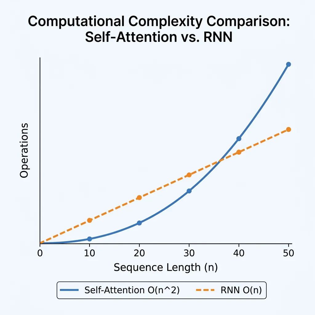
Adjust the sequence length to see how the number of operations (comparisons) grows quadratically for Self-Attention vs linearly for RNNs.
Looking Ahead: Beyond Quadratic Complexity
Having analyzed the complexity of the standard Transformer, we see that the attention mechanism is the primary bottleneck for scaling to long sequences.
The Race for Efficiency: This wall triggered a massive wave of research. To achieve linear complexity , numerous variants called ‘X-formers’ were proposed, such as the Linear Transformer, Performer, and Reformer. More recently, alternative architectures like State Space Models (e.g., Mamba) have emerged as strong contenders to replace Transformers for long-sequence tasks by achieving linear scaling without attention.
As we move to the next chapters, consider these questions:
- How can we modify the attention mechanism to achieve linear complexity ?
- Can we use external memory or compression to handle infinite sequences?
- How do modern models like Gemini or Claude handle million-token contexts?
These questions lead us to the exploration of efficient Transformers and alternative architectures in the coming chapters.
Quizzes
Quiz 1: When is Self-Attention computationally cheaper than a Recurrent layer?
Self-Attention is cheaper when the sequence length is smaller than the representation dimension (). In early NLP tasks, sentences were short (e.g., ) and embeddings were relatively large (e.g., ), making self-attention very efficient.
Quiz 2: What is the main bottleneck of Transformers when dealing with extremely long sequences (e.g., 100k tokens)?
The bottleneck is the time and memory complexity of the self-attention mechanism. As grows, the size of the attention matrix () grows quadratically, leading to massive memory consumption and compute requirements.
Quiz 3: Why do RNNs fail to utilize GPUs effectively compared to Transformers?
RNNs require sequential processing. To compute step , the output of step is required. This dependency prevents the model from processing all tokens in parallel. Transformers have sequential operations, allowing them to process all tokens at once, making full use of GPU parallelism.
Quiz 4: Why is the sequential complexity of RNNs while for Self-Attention it is ?
RNNs must process tokens one by one because the hidden state at step depends on the hidden state at step . This creates a sequential dependency of length . In Self-Attention, all pairs of tokens are compared in parallel, so all operations can be performed in a constant number of steps, , regardless of sequence length.
Quiz 5: In the complexity comparison table, what does represent in the Convolutional layer?
The variable represents the kernel size (or filter width) of the convolution. It determines how many adjacent tokens the convolutional layer looks at simultaneously.
References
- Vaswani, A., et al. (2017). Attention is all you need. Advances in neural information processing systems, 30. arXiv:1706.03762.