19.4 Sparse Autoencoders (SAE)

In the previous section, we used Probing Classifiers to detect specific concepts hidden in an LLM’s residual stream. However, probing is fundamentally a supervised, hypothesis-driven task: we can only find what we explicitly look for. If we want to discover the complete set of concepts a model has learned—without relying on human-provided labels—we need an unsupervised approach.

Over the past year, Sparse Autoencoders (SAEs) have emerged as the premier tool in mechanistic interpretability. They have successfully reverse-engineered the opaque, high-dimensional activations of state-of-the-art models like GPT-4 and Claude 3 Sonnet into millions of distinct, human-readable concepts.

1. The Superposition Hypothesis and Polysemanticity

If we want to understand what a neural network is “thinking,” the intuitive first step is to look at individual neurons. If a specific neuron fires every time the model processes the word “dog,” we might label it the “dog neuron.”

Unfortunately, this simple mapping fails in large language models. LLMs possess a finite number of dimensions in their residual stream (e.g., $d = 4096$ ), but they must represent millions of distinct concepts to understand human language. To solve this bottleneck, neural networks employ Superposition.

The Superposition Hypothesis suggests that models pack multiple unrelated concepts into the same representation space by utilizing almost-orthogonal vectors. Because high-dimensional spaces contain exponentially more almost-orthogonal directions than strictly orthogonal ones, the model can represent vastly more features than it has dimensions.

The side effect of superposition is that individual neurons become polysemantic. A single neuron might fire when processing the word “Apple” (the fruit), “Apple” (the tech company), and “Apple” (the record label). Looking at the raw neuron activation tells us nothing about which concept is currently active.

Superposition & Polysemanticity Simulator

See how 3 concepts are superimposed in 2 neurons (2D space).

Neuron Activations (ReLU)

Neuron 1

0.00

Neuron 2

0.00

Click the concept buttons to see activation patterns.

2. Dictionary Learning via Sparse Autoencoders

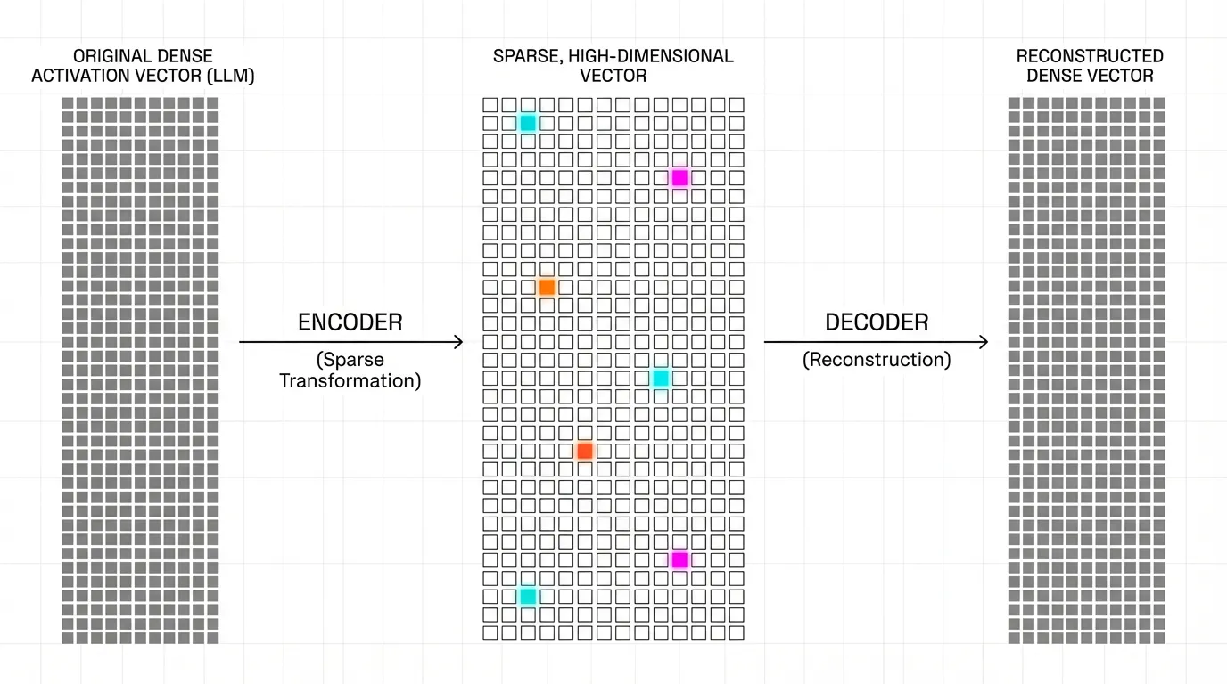
To untangle these polysemantic neurons, researchers treat the problem as Dictionary Learning. The goal is to find a set of sparse, overcomplete features (the dictionary) that linearly combine to form the model’s dense activation vectors.

A Sparse Autoencoder achieves this by projecting the $d$ -dimensional activation vector $x$ into a much larger $D$ -dimensional feature space $f$ (where $D \gg d$ , often 16x to 64x larger), and then reconstructing the original vector $\hat{x}$ .

sae_architecture Source: Generated by Gemini

The forward pass of a standard SAE is defined as:

$f = \text{ReLU}(W_{enc}(x - b_{pre}) + b_{enc})$ $\hat{x} = W_{dec} f + b_{dec} + b_{pre}$

To ensure the features are interpretable (monosemantic), we force the network to use only a tiny fraction of the $D$ features for any given input. This is typically enforced by adding an $L_1$ regularization penalty to the reconstruction loss:

$\mathcal{L} = ||x - \hat{x}||_2^2 + \lambda ||f||_1$

By expanding the dimension size and forcing sparsity, the SAE naturally decomposes polysemantic neurons into individual, single-meaning features.

3. The Dead Latent Problem

Training SAEs introduces severe engineering challenges. The most notorious is the Dead Latent (or Dead Neuron) problem.

Because the feature space $D$ is massive and the sparsity penalty ( $\lambda$ ) aggressively pushes activations to zero, many features in the SAE stop activating early in training. Once a feature stops activating, it receives zero gradient from the ReLU function, permanently trapping it in a “dead” state. In early SAE experiments, it was common for over 90% of the learned dictionary to be dead, wasting massive amounts of compute.

State-of-the-art training pipelines employ several techniques to revive these dead latents:

Ghost Gradients: Artificially routing gradients to dead neurons during the backward pass to give them a “nudge” toward useful directions.
Re-initialization: Periodically identifying dead neurons and resetting their encoder weights to match the dense activation vectors ( $x$ ) that currently have the highest reconstruction error.

4. Engineering the State-of-the-Art: Top-K SAEs

While the $L_1$ penalty enforces sparsity, it introduces a critical flaw: Shrinkage. The $L_1$ penalty constantly pulls all activations toward zero, meaning the SAE systematically underestimates the true magnitude of the features, degrading the reconstruction quality of $\hat{x}$ .

In 2024, OpenAI researchers demonstrated a breakthrough by scaling a 16-million latent SAE on GPT-4 activations [2]. To solve the shrinkage problem, they completely removed the $L_1$ penalty and replaced it with an explicit Top-K activation function.

Instead of relying on a loss penalty to push values to zero, a Top-K SAE simply computes the dense activations, strictly selects the $K$ highest values, and forcefully zeros out the rest. This directly controls the $L_0$ sparsity without distorting the activation magnitudes.

Here is how a Top-K SAE is implemented in PyTorch:

import torch
import torch.nn as nn
import torch.nn.functional as F

class TopKSAE(nn.Module):
    """
    Top-K Sparse Autoencoder (Gao et al., 2024).
    Replaces L1 regularization with an explicit Top-K activation function
    to solve the shrinkage problem and improve the sparsity-reconstruction frontier.
    """
    def __init__(self, d_model: int, d_sae: int, k: int):
        super().__init__()
        self.d_model = d_model
        self.d_sae = d_sae
        self.k = k
        
        # Initialize encoder and decoder weights
        # Decoder weights are typically unit-normalized in practice
        self.W_enc = nn.Parameter(torch.randn(d_model, d_sae) / (d_model ** 0.5))
        self.b_enc = nn.Parameter(torch.zeros(d_sae))
        
        self.W_dec = nn.Parameter(torch.randn(d_sae, d_model) / (d_sae ** 0.5))
        self.b_dec = nn.Parameter(torch.zeros(d_model))
        
        # Pre-encoder bias to center the activations
        self.b_pre = nn.Parameter(torch.zeros(d_model))

    def encode(self, x: torch.Tensor) -> torch.Tensor:
        # Center the input and project to high-dimensional feature space
        pre_acts = (x - self.b_pre) @ self.W_enc + self.b_enc
        acts = F.relu(pre_acts)
        
        # Explicit Top-K routing: keep only the top K activations, zero out the rest
        topk_vals, topk_indices = torch.topk(acts, self.k, dim=-1)
        
        # Reconstruct the sparse tensor
        sparse_acts = torch.zeros_like(acts)
        sparse_acts.scatter_(-1, topk_indices, topk_vals)
        
        return sparse_acts

    def decode(self, sparse_acts: torch.Tensor) -> torch.Tensor:
        # Project back to the original residual stream dimension
        return (sparse_acts @ self.W_dec) + self.b_dec + self.b_pre

    def forward(self, x: torch.Tensor) -> tuple[torch.Tensor, torch.Tensor]:
        sparse_acts = self.encode(x)
        x_reconstructed = self.decode(sparse_acts)
        return x_reconstructed, sparse_acts

# Example instantiation for a 4096-dim LLM residual stream
# Expanded to 131,072 features (32x expansion), keeping exactly 32 active
# sae = TopKSAE(d_model=4096, d_sae=131072, k=32)

5. Scaling Monosemanticity: The Golden Gate Claude

Anthropic applied SAEs to their production model, Claude 3 Sonnet, successfully extracting millions of highly abstract features [1]. Their findings fundamentally shifted how we view LLM representations.

They discovered that SAE features are concept-centric, not token-centric. For instance, a single feature representing the “Golden Gate Bridge” activates whether the model reads the English text “Golden Gate Bridge”, the Japanese translation “ゴールデンゲートブリッジ”, or even processes an image of the bridge.

golden_gate_claude Source: Generated by Gemini

More importantly, SAEs allow for causal steering. In a famous experiment, Anthropic researchers artificially clamped the activation of the Golden Gate Bridge feature to a high value during the model’s forward pass. The result was “Golden Gate Claude”—a model that became obsessively fixated on the bridge. When asked “How do I spend a day in London?”, the model suggested taking a flight to San Francisco to see the Golden Gate Bridge.

Beyond tourist attractions, researchers identified features for sycophancy, bias, scam emails, and dangerous capabilities (like generating bioweapons). By suppressing these specific features, SAEs offer a surgical approach to AI safety, allowing engineers to remove harmful behaviors without fine-tuning or degrading the model’s general intelligence.

6. Auto-Interp and Codebook Saturation

When an SAE extracts 16 million features, human evaluation becomes impossible. To scale interpretability, researchers use Automated Interpretability (Auto-Interp).

In Auto-Interp, a separate, powerful LLM (like GPT-4) acts as a judge. The judge is fed dozens of text snippets that maximally activate a specific SAE feature and prompted to determine what they have in common. The judge generates a label (e.g., “Legal terminology related to breach of contract”). To verify the label’s accuracy, the judge is then asked to predict how strongly the feature will activate on unseen text snippets.

One more speculative direction borrows ideas from qualitative analysis, especially codebook reduction and saturation, to ask whether an auto-interp workflow has stopped surfacing genuinely new categories [3]. This is better understood as an auditing heuristic for feature dictionaries than as proof that an SAE has exhausted every meaningful concept in the model.

8. Summary and Open Questions

Sparse Autoencoders have cracked open the black box. By expanding the LLM’s residual stream into a massive, sparse dictionary, we can map the chaotic superposition of polysemantic neurons into clean, single-meaning concepts. The shift from $L_1$ regularization to Top-K architectures has allowed these techniques to scale to frontier models like GPT-4 and Claude 3, enabling precise behavioral steering and safety interventions.

However, extracting features is only half the battle. If an LLM is a machine that “thinks,” features are merely the nouns and verbs of its thoughts. The next frontier in mechanistic interpretability is understanding how these features wire together to perform complex logic. How does the “If-Then” feature interact with the “Python Code” feature to generate a working script?

To answer this, we must map the Circuits of the LLM.

Quizzes

Quiz 1: Why do neural networks utilize superposition, leading to polysemantic neurons?

LLMs have a fixed, finite number of dimensions in their residual stream, but must represent millions of distinct linguistic and factual concepts. Superposition allows the model to pack multiple unrelated concepts into the same space using almost-orthogonal vectors, making individual neurons polysemantic (firing for multiple concepts).

Quiz 2: What is the fundamental trade-off when tuning the

\lambda

parameter for the

L_1

penalty in a standard SAE?

Increasing $\lambda$ improves the sparsity (and thus interpretability) of the features, but it worsens the reconstruction error (MSE) of the original activations. Furthermore, a high $L_1$ penalty causes “shrinkage,” artificially pulling all feature magnitudes toward zero.

Quiz 3: How does the Top-K SAE architecture solve the “shrinkage” problem inherent in standard

L_1

-regularized SAEs?

A Top-K SAE completely removes the $L_1$ penalty. Instead, it computes the dense activations, explicitly selects only the Top $K$ highest values, and forcefully zeros out the rest. This guarantees exact $L_0$ sparsity without applying a continuous mathematical penalty that shrinks the magnitude of the active features.

Quiz 4: What does the existence of “multilingual and multimodal” SAE features imply about the LLM’s internal representations?

It implies that the LLM is not merely memorizing surface-level token statistics or language-specific grammar. Instead, the model maps inputs into a deeply abstract, conceptual space where the fundamental “idea” of an object (like a bridge) is represented universally, regardless of the language or modality (text vs. image) used to invoke it.

Quiz 5: Formalize the exact mathematical gradient update logic sequence for Top-K routing inside an SAE during the backward pass. Define explicit Ghost Gradient boundaries to neutralize the Dead Latent problem.

A simple formalization treats Top-K routing as a hard mask $m_i = \mathbb{I}(i \in \text{Top-K}(x))$ , so the selected latent is $z_i = m_i x_i$ . In the backward pass, the direct gradient is masked in the same way: $\frac{\partial \mathcal{L}}{\partial x_i} \approx m_i \frac{\partial \mathcal{L}}{\partial z_i}$ . The dead-latent problem appears because units outside Top-K receive no direct learning signal. Ghost-gradient style fixes add an auxiliary reconstruction-based term to inactive latents, for example $g_i^{ghost} = \eta (1-m_i)\left(\frac{\partial \mathcal{L}}{\partial \hat{x}} W_{dec}^\top\right)_i$ , where $\eta$ is a small scaling factor. The key idea is not a universal boundary formula, but selectively giving inactive latents a weak gradient path so they can re-enter the active set later.

References

Templeton, A., et al. (2024). Scaling Monosemanticity: Extracting Interpretable Features from Claude 3 Sonnet. Transformer Circuits Thread. Link.
Gao, L., et al. (2024). Scaling and evaluating sparse autoencoders. arXiv:2406.04093.
De Paoli, S., & Mathis, W. S. (2025). Codebook Reduction and Saturation: Novel observations on Inductive Thematic Saturation for Large Language Models and initial coding in Thematic Analysis. arXiv:2503.04859.