5.1 Sparse vs Dense Models
The LLM inference economy has bifurcated. On one end, Mixture of Experts (MoE) models like DeepSeek-V3 and Qwen3 are the default choice for cloud-scale batch operations, code synthesis, and reasoning-heavy workloads. On the other end, Dense models remain the immovable standard for edge devices, mobile phones, and ultra-low-latency APIs where memory capacity is strictly capped.
To understand why sparsity has become a defining paradigm, we must first deconstruct the fundamental difference between dense and sparse architectures. This is not just a minor architectural tweak; it is a fundamental shift in how we allocate computational resources.
The Analogy: The Generalist vs. The Specialist Hospital
Imagine a Dense Model as a traditional, albeit highly capable, rural hospital. There is one brilliant “Super-Doctor” on staff. Whether a patient comes in with a paper cut, a broken leg, or a complex neurological disorder, this single Super-Doctor must examine the patient, consult their entire vast medical knowledge, and prescribe a treatment. As the hospital grows (scaling the model), the Super-Doctor learns more, but the line of patients out the door grows longer. Every patient requires the doctor’s full attention (all parameters are activated).
Now, imagine a Sparse MoE Model as a modern mega-hospital. When a patient walks in, they do not see the doctors immediately. Instead, they are greeted by a highly efficient Triage Nurse (the Router). The nurse takes one look at the patient’s symptoms and instantly routes them to the exact specialists needed—perhaps the Cardiologist and the Neurologist (the Experts). The hospital employs hundreds of doctors (massive total parameter count), but for any given patient, only two doctors are actively working (small active parameter count). This allows the hospital to process thousands of patients simultaneously with unparalleled specialized knowledge, without the computational bottleneck of a single doctor doing everything.
The Scaling Crisis and the MoE Revival
Historically, Dense Transformer models dominated due to their simplicity and predictable scaling laws. If you wanted a smarter model, you trained a larger dense network. However, this single-minded pursuit of scale led directly to a computational cliff.
Training and serving a state-of-the-art dense model—where every single parameter is activated to process every single token—is an undertaking of astronomical proportions. A 400-billion parameter dense model requires computing 400 billion multiply-accumulate operations per token.
The concept of MoE actually predates the Transformer. The true watershed moment arrived in 2017 with a Google Brain paper by Noam Shazeer et al., titled “Outrageously Large Neural Networks: The Sparsely-Gated Mixture-of-Experts Layer” [1]. However, the hardware of 2017 was not ready for the complex memory access patterns of MoE. It remained a fascinating academic curiosity until Mistral AI released Mixtral 8x7B in early 2024, proving that sparse open-weight models could destroy dense models of similar compute classes [2].
Recent models like DeepSeek-V3 (671B total parameters, 37B active) and Llama 4 Maverick (400B total, 17B active) have made MoE a common design choice among frontier-scale models, especially when capacity and inference compute need to be decoupled [3].
The Mathematics of Sparsity
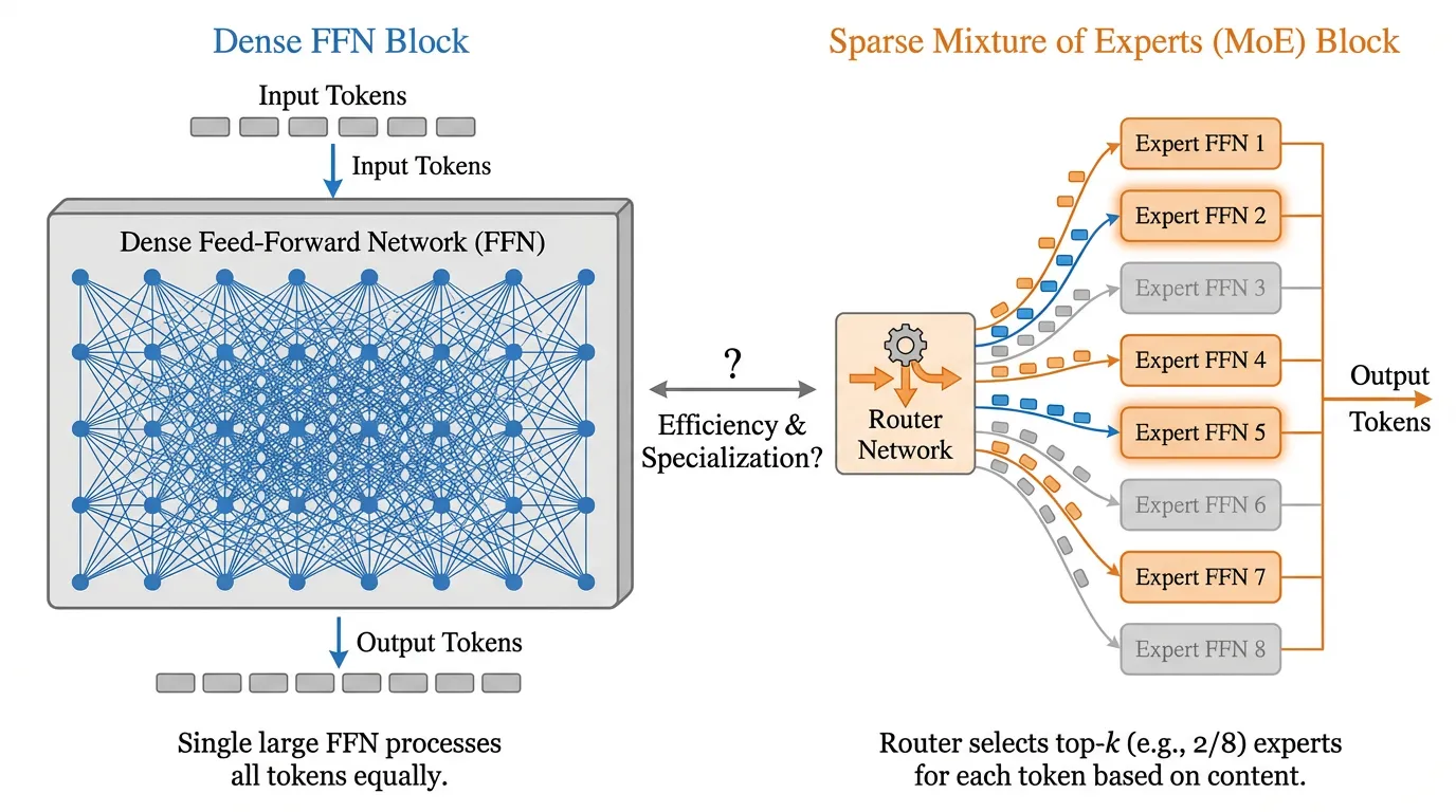
In a standard Dense Transformer, the Feed-Forward Network (FFN) applies the same massive weight matrices to every token in the sequence:
In a Sparse MoE architecture, the dense FFN is replaced by a set of independent FFNs, called Experts, and a Gating Network (or Router) that determines which experts process which tokens.
The output of the MoE layer for a given token is the weighted sum of the outputs of the selected experts:
Where:
- is the total number of experts.
- is the output of the -th expert network.
- is the gating value (routing weight) for the -th expert.
The Routing Mechanism (Top-K)
To achieve sparsity, the gating network must output a sparse vector (mostly zeros). The most common approach is Top-K Routing. The router projects the token representation into logits, applies a Softmax, and keeps only the top values, setting the rest to zero:
If (as in many top-2 MoE designs such as Mixtral), only the top 2 experts out of are activated for that specific token.
 Source: Generated by Gemini
Total vs. Active Parameters: The Efficiency Arithmetic
The most misunderstood aspect of MoE models is the parameter count. When you read that DeepSeek-V3 is a “671B parameter model,” you must split this into two metrics:
- Total Parameters (Capacity): The sheer volume of knowledge the model has memorized. All 671 billion parameters must reside in VRAM.
- Active Parameters (Compute): The number of parameters used during the forward pass for a single token. For DeepSeek-V3, this is only 37 billion.
Why does this matter? In large-batch inference (e.g., processing a massive prompt or serving thousands of users simultaneously), the bottleneck is arithmetic (FLOPs). A dense 671B model would require ~1.34 teraFLOPs per token. DeepSeek-V3 only requires ~74 gigaFLOPs per token. This translates to a ~94% reduction in compute cost per token, allowing cloud providers to serve massive models at a fraction of the cost.
Dense vs. Sparse: Engineering Trade-offs
Neither architecture is universally superior. The optimal choice depends entirely on your deployment constraints.
| Feature | Dense Models (e.g., Llama 3 70B) | Sparse MoE Models (e.g., DeepSeek-V3, Qwen3) |
|---|---|---|
| Compute (FLOPs) | High (Proportional to total size) | Low (Proportional to active size) |
| Memory (VRAM) | High (Proportional to total size) | Extremely High (Must store all experts in VRAM) |
| Inference Latency | Highly predictable | Variable (Depends on routing overhead and batch size) |
| VRAM Bandwidth | Efficient (Sequential reads) | Bottlenecked (Random access to scattered experts) |
| Training Stability | Very stable | Prone to “Expert Collapse” (requires load-balancing) |
| Best Use Case | Edge devices, mobile, latency-critical APIs | Cloud-scale batch inference, complex reasoning, coding |
Implementation: Building a Sparse MoE Layer in PyTorch
To truly understand the mechanics, let’s implement a standard Top-2 MoE layer. While production models use highly optimized custom CUDA kernels (like Triton or Megatron-LM’s scatter/gather operations) to avoid moving memory around, this PyTorch implementation demonstrates the exact mathematical forward pass.
import torch
import torch.nn as nn
import torch.nn.functional as F

class Expert(nn.Module):
    """A standard Feed-Forward Network acting as a single expert."""
    def __init__(self, d_model, d_ff):
        super().__init__()
        self.w1 = nn.Linear(d_model, d_ff, bias=False)
        self.w2 = nn.Linear(d_ff, d_model, bias=False)
        self.act = nn.SiLU()

    def forward(self, x):
        return self.w2(self.act(self.w1(x)))

class SparseMoELayer(nn.Module):
    """A Top-K Sparse Mixture of Experts Layer."""
    def __init__(self, d_model, d_ff, num_experts, top_k):
        super().__init__()
        self.num_experts = num_experts
        self.top_k = top_k

        # The Router (Gating Network)
        self.router = nn.Linear(d_model, num_experts, bias=False)

        # The Experts
        self.experts = nn.ModuleList([
            Expert(d_model, d_ff) for _ in range(num_experts)
        ])

    def forward(self, x):
        # x shape: (batch_size, seq_len, d_model)
        batch_size, seq_len, d_model = x.shape
        x_flat = x.view(-1, d_model) # Flatten to (batch * seq_len, d_model)

        # 1. Calculate Routing Logits
        router_logits = self.router(x_flat) # (batch * seq_len, num_experts)
        routing_weights = F.softmax(router_logits, dim=-1)

        # 2. Select Top-K Experts
        top_k_weights, top_k_indices = torch.topk(routing_weights, self.top_k, dim=-1)

        # Normalize weights among the selected top-k experts so they sum to 1
        top_k_weights = top_k_weights / top_k_weights.sum(dim=-1, keepdim=True)

        # 3. Dispatch tokens to experts and aggregate
        final_output = torch.zeros_like(x_flat)

        # Iterate through each expert (Pedagogical approach; slow in pure PyTorch)
        for i, expert in enumerate(self.experts):
            # Find which tokens were routed to expert `i`
            expert_mask = (top_k_indices == i).any(dim=-1)

            if not expert_mask.any():
                continue # Skip if no tokens were routed to this expert

            # Extract the actual tokens
            expert_tokens = x_flat[expert_mask]

            # Forward pass through the specific expert
            expert_out = expert(expert_tokens)

            # Extract the corresponding routing weights for these tokens
            # We need to find the exact position (0 to top_k-1) where this expert was selected
            weight_mask = top_k_indices[expert_mask] == i
            expert_weights = top_k_weights[expert_mask][weight_mask].unsqueeze(-1)

            # Scale output by the routing weight and add to the final output tensor
            token_indices = expert_mask.nonzero(as_tuple=True)[0]
            final_output[token_indices] += expert_out * expert_weights

        return final_output.view(batch_size, seq_len, d_model)

# Example Usage
d_model = 1024
layer = SparseMoELayer(d_model=d_model, d_ff=4096, num_experts=8, top_k=2)
dummy_input = torch.randn(2, 128, d_model) # Batch 2, Seq 128
output = layer(dummy_input)
print(f"Output shape: {output.shape}") # Expected: [2, 128, 1024]
Interactive Visualization: Token Routing
To conceptualize how tokens scatter across experts, consider the following interactive visualizer. Observe how different semantic tokens are routed to specific experts.
MoE Routing Debugger (Top-2)
Hover over a token to see which experts are activated.
(Note: In a real engineering environment, you would log the top_k_indices from the PyTorch model and pipe them into a visualization dashboard to ensure no single expert is being overloaded.)
Looking Ahead
We have established that MoE decouples model capacity from inference compute. However, the code implementation above hides a massive systemic risk: What happens if the router sends 99% of the tokens to Expert 0?
If one expert receives all the traffic, the hardware executing that expert will bottleneck, while the GPUs holding the other experts sit idle. This catastrophic failure mode is known as Expert Collapse. In the next section, 5.2 Routing Algorithms, we will explore the advanced loss functions and auxiliary-loss-free routing mechanisms designed to keep the experts perfectly balanced.
Quizzes
Quiz 1: If an MoE model has 671B total parameters and only 37B active parameters per token, why can’t we run it on a single 80GB GPU, given that 37B parameters in FP16 easily fit into 80GB of VRAM?
Because the routing mechanism is dynamic and unpredictable at the sequence level. The router decides which experts to activate on a per-token basis at runtime. Therefore, the weights for all 671B parameters must reside in VRAM simultaneously so they are instantly available when called upon. Swapping experts from CPU RAM to GPU VRAM on the fly would introduce unacceptable PCIe latency overhead. MoE reduces compute (FLOPs) and activation memory, but it does not reduce the static model weight VRAM requirements.
Quiz 2: In a Top-2 routing setup, what happens if the router assigns an overwhelming majority of tokens in a sequence to Expert 1, leaving the other experts completely idle?
This phenomenon is known as “expert collapse” or a load-balancing failure. If Expert 1 processes all tokens, it becomes a severe computational bottleneck, destroying the parallelization benefits of MoE. In a distributed setup (Expert Parallelism), the GPU hosting Expert 1 will be overloaded and OOM (Out of Memory), while other GPUs sit idle waiting for synchronization. This is why modern MoE architectures require sophisticated load-balancing algorithms, which we will cover in the next section.
Quiz 3: For a mobile phone deployment (e.g., an on-device AI assistant), would you prefer a 7B Dense model or a 40B MoE model with 7B active parameters? Justify your engineering choice.
The 7B Dense model is heavily preferred for edge deployment. Edge devices (like smartphones) are severely constrained by RAM capacity and memory bandwidth, not just compute. A 40B MoE model requires storing 40B parameters in memory, which exceeds the unified RAM capacity of almost all mobile devices. Furthermore, the dynamic routing overhead and unpredictable memory access patterns of MoE are hostile to the constrained, highly deterministic architectures of mobile NPUs (Neural Processing Units).
References
- Shazeer, N., et al. (2017). Outrageously Large Neural Networks: The Sparsely-Gated Mixture-of-Experts Layer. arXiv:1701.06538.
- Jiang, A. Q., et al. (2024). Mixtral of Experts. arXiv:2401.04088.
- DeepSeek-AI. (2024). DeepSeek-V3 Technical Report. arXiv:2412.19437.