6.3 Large-scale Training Stability

Training a 1B parameter model is like driving a sports car on a closed track; you might spin out, but recovery is easy. Training a 100B+ parameter model across tens of thousands of GPUs is like flying a supersonic jet. A microscopic anomaly—a corrupted batch of data, a slight numerical overflow in a single attention head, or a sudden gradient variance—can trigger a catastrophic failure known as a Loss Spike.

Historically, large-scale training was heavily reactive. During the training of models like OPT-175B or early LLaMA iterations, engineers had to monitor dashboards 24/7. When a loss spike occurred, the standard operating procedure was to pause training, roll back to a checkpoint from a few hundred steps prior, skip the offending data batch, and restart. This “rollback tax” wasted millions of dollars in idle GPU compute.

By 2024-2025, the paradigm shifted toward proactive (or passive) stability. State-of-the-art models like DeepSeek-V3 [1] achieved a remarkable engineering milestone: zero irrecoverable loss spikes and zero rollbacks throughout the training of 14.8 trillion tokens, even while utilizing aggressive FP8 mixed precision.

This section dives into the anatomy of training instability and the architectural interventions required to keep multi-billion parameter models well-conditioned from initialization to convergence.

1. The Anatomy of a Loss Spike

To prevent instability, we must first understand its mechanical origin. A loss spike is rarely instantaneous; it is the terminal symptom of a silent, compounding numerical disease.

Recent analyses [2] have shown that training divergence is almost always preceded by the uncontrolled growth of $L_2$ norms in the outputs of specific linear layers—namely the Query/Key projections, the output Projection layer, and the second Fully Connected layer (FC2) in the Feed-Forward Network.

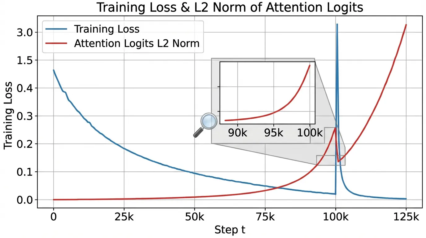
The Logit Growth Problem

As training progresses, the model becomes more confident. To minimize the cross-entropy loss, the network pushes the logits of the correct tokens to extreme positive values.

1. Attention Saturation: If the $L_2$ norm of the Query and Key vectors grows unchecked, the dot product $Q \cdot K^T$ produces massive scalars.
2. Softmax Collapse: When these massive scalars are passed through the softmax function, the distribution collapses into a near one-hot vector (e.g., [0.0001, 0.9998, 0.0001]).
3. Gradient Starvation & Explosion: The gradients for the non-target tokens vanish, while the gradient for the target token becomes hyper-sensitive. A single noisy or out-of-distribution token in the next batch will generate an astronomical gradient, which propagates backward, corrupting the momentum buffers in the AdamW optimizer and permanently destroying the weight distributions.

2. Architectural Stabilizers

Rather than relying on hyperparameter tuning (like lowering the learning rate, which hurts final performance), modern foundation models modify the architecture to strictly bound internal activations.

2.1 QK Layer Normalization

Standard Transformers apply LayerNorm (or RMSNorm) to the input of the attention block. However, the $Q$ and $K$ projections can still drift. By applying an additional normalization directly to the Query and Key vectors before the dot product, we force the attention logits to be strictly bounded by the hidden dimension size.

This prevents the attention entropy from collapsing, allowing engineers to safely increase the learning rate by up to 1.5x without divergence [2].

2.2 Softmax Capping (Logit Capping)

Even with QK Norm, the final logits fed into the cross-entropy loss can grow too large. Models like Gemma and Grok utilize Softmax Capping, which bounds the pre-softmax logits to a fixed range $[-c, c]$ using a scaled hyperbolic tangent function.

Typically, $c$ is set to a value like 30.0. In the linear region of $\tanh$ (near zero), the gradients flow normally. As logits approach $c$, the gradient naturally decays, acting as an automatic, differentiable gradient clipper that prevents the model from becoming overconfident.

2.3 The $z$-loss (Auxiliary Logit Penalty)

Introduced during the training of PaLM [3], the $z$-loss is an auxiliary objective added to the primary cross-entropy loss. It penalizes the logarithm of the partition function (the denominator of the softmax), encouraging the maximum logit to remain close to zero.

Where $\alpha$ is typically a very small constant (e.g., $10^{-4}$). This prevents the exponential moving averages in the optimizer from being corrupted by massive logit gradients.

3. Engineering Stable PyTorch Components

Let’s implement these stability mechanisms in a realistic PyTorch setting. The following code demonstrates a robust Attention layer and a custom Cross-Entropy loss function designed for 100B+ scale training.

import torch
import torch.nn as nn
import torch.nn.functional as F

class RMSNorm(nn.Module):
    def __init__(self, dim: int, eps: float = 1e-6):
        super().__init__()
        self.eps = eps
        self.weight = nn.Parameter(torch.ones(dim))

    def forward(self, x):
        variance = x.pow(2).mean(-1, keepdim=True)
        x_norm = x * torch.rsqrt(variance + self.eps)
        return self.weight * x_norm

class StableAttention(nn.Module):
    def __init__(self, d_model: int, num_heads: int, logit_cap: float = 30.0):
        super().__init__()
        self.num_heads = num_heads
        self.head_dim = d_model // num_heads
        self.logit_cap = logit_cap
        
        self.q_proj = nn.Linear(d_model, d_model, bias=False)
        self.k_proj = nn.Linear(d_model, d_model, bias=False)
        self.v_proj = nn.Linear(d_model, d_model, bias=False)
        self.o_proj = nn.Linear(d_model, d_model, bias=False)
        
        # Stability: QK Normalization
        self.q_norm = RMSNorm(self.head_dim)
        self.k_norm = RMSNorm(self.head_dim)

    def forward(self, x):
        B, L, D = x.size()
        
        q = self.q_proj(x).view(B, L, self.num_heads, self.head_dim).transpose(1, 2)
        k = self.k_proj(x).view(B, L, self.num_heads, self.head_dim).transpose(1, 2)
        v = self.v_proj(x).view(B, L, self.num_heads, self.head_dim).transpose(1, 2)
        
        # Apply RMSNorm to Q and K independently per head
        q = self.q_norm(q)
        k = self.k_norm(k)
        
        # Scaled Dot-Product
        scores = torch.matmul(q, k.transpose(-2, -1)) / (self.head_dim ** 0.5)
        
        # Stability: Softmax Capping (Logit Capping)
        if self.logit_cap > 0:
            scores = self.logit_cap * torch.tanh(scores / self.logit_cap)
            
        attn_weights = F.softmax(scores, dim=-1)
        out = torch.matmul(attn_weights, v)
        
        out = out.transpose(1, 2).contiguous().view(B, L, D)
        return self.o_proj(out)

def cross_entropy_with_zloss(logits: torch.Tensor, targets: torch.Tensor, z_loss_weight: float = 1e-4):
    """
    Computes Cross Entropy Loss with an auxiliary z-loss to prevent logit drift.
    """
    # Standard Cross Entropy
    ce_loss = F.cross_entropy(logits.view(-1, logits.size(-1)), targets.view(-1))
    
    # Compute z-loss: log^2(sum(exp(logits)))
    # We use logsumexp for numerical stability
    log_z = torch.logsumexp(logits, dim=-1)
    z_loss = (log_z ** 2).mean()
    
    return ce_loss + (z_loss_weight * z_loss)

4. Advanced Stability: MoE and Decoupling

Auxiliary-Loss-Free Load Balancing

In Mixture-of-Experts (MoE) models, routing tokens to experts unevenly causes hardware bottlenecks (expert collapse). Historically, an auxiliary loss was added to the training objective to force even distribution. However, this auxiliary loss physically alters the model’s gradients, often conflicting with the language modeling objective and causing instability.

DeepSeek-V3 [1] introduced Auxiliary-Loss-Free Load Balancing. Instead of modifying the loss function, they dynamically adjust a bias term added to the routing logits. Crucially, this bias is mathematically detached from the gradient tape (bias.detach()). The routing mechanism achieves perfect balance during the forward pass, but the backward pass only updates the router weights based on pure token-expert affinity, entirely eliminating a major source of MoE training divergence.

Scale-Distribution Decoupling (SDD)

In very deep Post-Norm architectures, the variance of the residual stream grows linearly with depth, leading to gradient explosion. Wang et al. (2025) proposed Scale-Distribution Decoupling (SDD) [4]. SDD explicitly separates the scale (magnitude) and distribution (direction) of weight matrices in fully-connected layers. By applying a normalization mechanism directly to the pre-activations and relying on a learnable scaling vector, SDD ensures that gradients remain well-conditioned, allowing Post-Norm Transformers to scale stably without needing complex initialization tricks.

5. Interactive: The Loss Spike Simulator

To build intuition for how these architectural choices prevent divergence, interact with the simulator below. It models the internal $L_2$ norm growth of a hypothetical training run. Notice how enabling QK-Norm and Softmax Capping acts as a “shock absorber” against noisy data batches.

6. Mixed Precision (FP8) Stability

As models scale to the trillion-parameter regime, training in BF16 becomes bottlenecked by memory bandwidth. The industry is aggressively moving to FP8 (8-bit floating point) mixed precision.

FP8 severely restricts dynamic range (the maximum representable value is 448 in E4M3 format). If the $L_2$ norms of activations grow, they will immediately overflow FP8 bounds, resulting in NaN gradients.

To train stably in FP8, modern frameworks employ Fine-grained Quantization. Instead of quantizing an entire tensor with a single scale factor, tensors are blocked (e.g., $1 \times 128$ tiles), and each block receives its own FP32 scale factor. Furthermore, critical “bottleneck” tensors—such as the latent vectors in Multi-head Latent Attention (MLA)—are kept in higher precision (BF16) because their variance is too high for FP8 to capture without catastrophic information loss.

Summary and Next Steps

Stability is no longer a dark art of hyperparameter tuning; it is a rigorous architectural discipline. By strictly controlling the magnitude of internal representations via QK Norm, Softmax Capping, and decoupled routing, engineers can safely push learning rates higher and utilize aggressive low-precision formats like FP8.

With the model architecture now stable, the next challenge is mapping this massive computational graph onto physical hardware. In Chapter 7: Training Optimization & Systems, we will explore how 3D Parallelism, ZeRO optimization, and Flash Attention physically distribute these stable matrices across tens of thousands of GPUs.

Quizzes

References

1. DeepSeek-AI. (2024). DeepSeek-V3 Technical Report. arXiv:2412.19437.
2. Anonymous. (2024). Methods of Improving LLM Training Stability. arXiv:2410.16682.
3. Chowdhery, A., et al. (2022). PaLM: Scaling Language Modeling with Pathways. arXiv:2204.02311.
4. Wang, Y., Zhuo, Z., Zeng, Y., Zhou, X., Yang, J., & Li, X. (2025). Scale-Distribution Decoupling: Enabling Stable and Effective Training of Large Language Models. arXiv:2502.15499.